Visualizing survey data

NoteLearning objectives

• Identify methods for importing survey datasets
• Estimate summary statistics using survey weights
• Import and wrangle messy data from top-line survey reports
• Design bar charts for reporting Likert scale data
• Evaluate the interpretability of various bar charts

Reporting on public opinion

A brief history of polling

A poll is a survey or inquiry into public opinion conducted by interviewing a random sample of people.

The modern era of public opinion polling began with George Gallup’s 1936 presidential election prediction. Gallup’s probability-based sample of 3,000 correctly predicted Franklin Roosevelt’s victory while Literary Digest’s 10-million-postcard straw poll predicted the opposite. The lesson — that representativeness matters more than sample size — shaped polling practice for the next century.

Telephone polling with random-digit dialing (RDD) dominated from the 1970s through the 2000s, reaching landline households at reasonable cost. As landline use collapsed, response rates fell from ~35% in the mid-1990s to under 10% by the 2010s. Most major pollsters now use probability-based online panels — pre-recruited, demographically stratified samples — as their primary mode.

Sources of public opinion data

Most public opinion data is proprietary — firms collect it for clients and publish only summary results. Some academic and government datasets are publicly available:

• American National Election Studies (ANES) — biennial pre/post-election surveys dating to 1948
• General Social Survey (GSS) — annual sociological survey since 1972
• Nationscape — large weekly surveys of US political opinion from 2019–2021
• Roper iPoll — archive of over 700,000 survey questions from hundreds of organizations

Common challenges

Working with survey datasets introduces three recurring challenges:

1. File formats: Academic survey files are typically distributed in Stata (.dta) or SPSS (.sav) format, not CSV.
2. Encoded missing values: Surveys encode non-responses (e.g., “Refused”, “Not asked”) with numeric codes that must be treated as missing, not as valid data.
3. Survey weights: Most surveys oversample some demographic groups and undersample others to manage cost. Weights adjust for these imbalances when estimating population-level statistics.

Importing and wrangling survey data

Importing Stata files with {haven}

The {haven} package reads Stata, SPSS, and SAS files:

library(haven)

nationscape <- read_dta(file = "data/ns20210112.dta")
nationscape

# A tibble: 4,138 × 234
   response_id start_date          right_track        economy_better interest registration
   <chr>       <dttm>              <dbl+lbl>          <dbl+lbl>      <dbl+lb> <dbl+lbl>   
 1 07700007    2021-01-12 10:52:22   2 [Off on the w… 1 [Better]      1 [Mos…   1 [Regist…
 2 07700008    2021-01-12 10:55:11   1 [Generally he… 1 [Better]     NA         1 [Regist…
 3 07700009    2021-01-12 10:50:00   2 [Off on the w… 2 [About the …  2 [Som…   1 [Regist…
 4 07700010    2021-01-12 10:47:32   2 [Off on the w… 2 [About the …  1 [Mos…   1 [Regist…
 5 07700011    2021-01-12 10:52:57   2 [Off on the w… 3 [Worse]       3 [Onl… 999 [Don't …
 6 07700013    2021-01-12 10:50:17 999 [Not sure]     1 [Better]      2 [Som…   1 [Regist…
 7 07700014    2021-01-12 10:49:44 999 [Not sure]     3 [Worse]       2 [Som…   1 [Regist…
 8 07700015    2021-01-12 10:51:21 999 [Not sure]     3 [Worse]       2 [Som…   1 [Regist…
 9 07700016    2021-01-12 11:01:55   1 [Generally he… 2 [About the …  2 [Som…   1 [Regist…
10 07700020    2021-01-12 10:58:21   2 [Off on the w… 2 [About the …  4 [Har…   1 [Regist…
# ℹ 4,128 more rows
# ℹ 228 more variables: news_sources_facebook <dbl+lbl>, news_sources_cnn <dbl+lbl>,
#   news_sources_msnbc <dbl+lbl>, news_sources_fox <dbl+lbl>,
#   news_sources_network <dbl+lbl>, news_sources_localtv <dbl+lbl>,
#   news_sources_telemundo <dbl+lbl>, news_sources_npr <dbl+lbl>,
#   news_sources_amtalk <dbl+lbl>, news_sources_new_york_times <dbl+lbl>,
#   news_sources_local_newspaper <dbl+lbl>, news_sources_other <dbl+lbl>, …

Stata files store variable labels alongside numeric codes. The tibble output above shows the numeric codes; to work with the labels, convert using as_factor().

Converting labels to factors

nationscape <- as_factor(nationscape)
nationscape

1

as_factor() replaces each labeled numeric column with a factor whose levels match the Stata value labels. This makes the data readable and prevents accidental numeric interpretation of categorical codes.

# A tibble: 4,138 × 234
   response_id start_date          right_track        economy_better interest registration
   <chr>       <dttm>              <fct>              <fct>          <fct>    <fct>       
 1 07700007    2021-01-12 10:52:22 Off on the wrong … Better         Most of… Registered  
 2 07700008    2021-01-12 10:55:11 Generally headed … Better         <NA>     Registered  
 3 07700009    2021-01-12 10:50:00 Off on the wrong … About the same Some of… Registered  
 4 07700010    2021-01-12 10:47:32 Off on the wrong … About the same Most of… Registered  
 5 07700011    2021-01-12 10:52:57 Off on the wrong … Worse          Only no… Don't know  
 6 07700013    2021-01-12 10:50:17 Not sure           Better         Some of… Registered  
 7 07700014    2021-01-12 10:49:44 Not sure           Worse          Some of… Registered  
 8 07700015    2021-01-12 10:51:21 Not sure           Worse          Some of… Registered  
 9 07700016    2021-01-12 11:01:55 Generally headed … About the same Some of… Registered  
10 07700020    2021-01-12 10:58:21 Off on the wrong … About the same Hardly … Registered  
# ℹ 4,128 more rows
# ℹ 228 more variables: news_sources_facebook <fct>, news_sources_cnn <fct>,
#   news_sources_msnbc <fct>, news_sources_fox <fct>, news_sources_network <fct>,
#   news_sources_localtv <fct>, news_sources_telemundo <fct>, news_sources_npr <fct>,
#   news_sources_amtalk <fct>, news_sources_new_york_times <fct>,
#   news_sources_local_newspaper <fct>, news_sources_other <fct>,
#   news_sources_other_TEXT <chr>, pres_approval <fct>, vote_2016 <fct>, …

Estimating proportions without weights

A simple unweighted cross-tabulation of college education by party identification:

nationscape |>
  count(college, pid3) |>
  drop_na() |>
  mutate(pct = n / sum(n), .by = pid3) |>
  select(-n) |>
  pivot_wider(names_from = pid3, values_from = pct)

1

count() tabulates all combinations of college and pid3.

2

drop_na() removes respondents who were not asked one or both questions.

3

mutate(pct = n / sum(n), .by = pid3) computes within-party proportions.

# A tibble: 3 × 5
  college  Democrat Republican Independent `Something else`
  <fct>       <dbl>      <dbl>       <dbl>            <dbl>
1 Agree       0.704      0.349       0.487            0.445
2 Disagree    0.148      0.487       0.308            0.264
3 Not Sure    0.149      0.164       0.205            0.291

This is fast but ignores the survey’s sampling design. The proportions will be biased if some demographic groups were oversampled.

Survey weights

The Nationscape dataset includes a weight variable:

nationscape |> select(weight)

# A tibble: 4,138 × 1
   weight
    <dbl>
 1 2.17  
 2 3.61  
 3 5.01  
 4 0.969 
 5 0.173 
 6 0.153 
 7 0.924 
 8 0.144 
 9 0.0964
10 2.64  
# ℹ 4,128 more rows

A weight greater than 1 means that respondent represents more people in the population than they do in the sample (their group was undersampled). A weight less than 1 means their group was oversampled.

Weighted estimation with {srvyr}

The {srvyr} package applies survey weights to dplyr-style operations. First, declare the survey design:

library(srvyr)

ns_design <- nationscape |>
  as_survey_design(ids = 1, weights = weight)
ns_design

1

ids = 1 indicates a simple random sample (no clustering by household or geography). weights = weight specifies the weight column.

Independent Sampling design (with replacement)
Called via srvyr
Sampling variables:
  - ids: `1` 
  - weights: weight 
Data variables: 
  - response_id (chr), start_date (dttm), right_track (fct), economy_better (fct),
    interest (fct), registration (fct), news_sources_facebook (fct), news_sources_cnn
    (fct), news_sources_msnbc (fct), news_sources_fox (fct), news_sources_network (fct),
    news_sources_localtv (fct), news_sources_telemundo (fct), news_sources_npr (fct),
    news_sources_amtalk (fct), news_sources_new_york_times (fct),
    news_sources_local_newspaper (fct), news_sources_other (fct), news_sources_other_TEXT
    (chr), pres_approval (fct), vote_2016 (fct), vote_2016_other_text (chr),
    vote_intention_retro (fct), vote_2020_retro (fct), vote_2020_retro_other_text (chr),
    who_won (fct), who_won_other_text (chr), primary_party_retro (fct),
    group_favorability_whites (fct), group_favorability_blacks (fct),
    group_favorability_latinos (fct), group_favorability_asians (fct),
    group_favorability_evangelicals (fct), group_favorability_socialists (fct),
    group_favorability_muslims (fct), group_favorability_labor_unions (fct),
    group_favorability_the_police (fct), group_favorability_undocumented (fct),
    group_favorability_lgbt (fct), group_favorability_republicans (fct),
    group_favorability_democrats (fct), group_favorability_white_men (fct),
    group_favorability_jews (fct), group_favorability_blm (fct),
    group_favorability_trump_s (fct), group_favorability_biden_s (fct),
    cand_favorability_trump (fct), cand_favorability_obama (fct), cand_favorability_biden
    (fct), cand_favorability_harris (fct), cand_favorability_pence (fct), rep_prim_vote
    (fct), rep_prim_vote_TEXT (chr), dem_prim_vote (fct), dem_prim_vote_TEXT (chr),
    house_intent_retro (fct), senate_intent_retro (fct), governor_intent_retro (fct),
    primary_sen_barrasso (fct), primary_sen_blackburn (fct), primary_sen_blunt (fct),
    primary_sen_boozman (fct), primary_sen_crapo (fct), primary_sen_cruz (fct),
    primary_sen_fischer (fct), primary_sen_grassley (fct), primary_sen_hoeven (fct),
    primary_sen_lankford (fct), primary_sen_lee (fct), primary_sen_moran (fct),
    primary_sen_murkowski (fct), primary_sen_neelykennedy (fct), primary_sen_paul (fct),
    primary_sen_portman (fct), primary_sen_rubio (fct), primary_sen_scott_tim (fct),
    primary_sen_shelby (fct), primary_sen_thune (fct), primary_sen_toomey (fct),
    primary_sen_wicker (fct), primary_sen_young (fct), primary_sen_braun (fct),
    primary_sen_cramer (fct), primary_sen_hawley (fct), primary_sen_romney (fct),
    primary_sen_scott_rick (fct), cand_truth_donald_trump (fct), cand_truth_joe_biden
    (fct), cand_facts_donald_trump (fct), cand_facts_joe_biden (fct), pence_president
    (fct), racial_attitudes_tryhard (fct), racial_attitudes_generations (fct),
    racial_attitudes_marry (fct), racial_attitudes_date (fct), gender_attitudes_maleboss
    (fct), gender_attitudes_logical (fct), gender_attitudes_opportunity (fct),
    gender_attitudes_complain (fct), discrimination_blacks (fct), discrimination_whites
    (fct), discrimination_muslims (fct), discrimination_christians (fct),
    discrimination_jews (fct), discrimination_women (fct), discrimination_men (fct),
    discrimination_asians (fct), discrimination_latinos (fct), sen_knowledge (fct),
    sc_knowledge (fct), pid3 (fct), pid7 (fct), pid7_legacy (fct), strength_democrat
    (fct), strength_republican (fct), lean_independent (fct), ideo5 (fct), employment
    (fct), employment_other_text (chr), work_location (fct), foreign_born (fct), language
    (fct), religion (fct), religion_other_text (chr), is_evangelical (fct),
    orientation_group (fct), in_union (fct), married (fct), extra_n_children (dbl),
    household_gun_owner (fct), wall (fct), cap_carbon (fct), guns_bg (fct), mctaxes
    (fct), estate_tax (fct), raise_upper_tax (fct), college (fct), abortion_any_time
    (fct), abortion_never (fct), abortion_conditions (fct), late_term_abortion (fct),
    abolish_priv_insurance (fct), abortion_insurance (fct), abortion_waiting (fct),
    china_tariffs (fct), criminal_immigration (fct), environment (fct), guaranteed_jobs
    (fct), green_new_deal (fct), gun_registry (fct), immigration_insurance (fct),
    immigration_separation (fct), immigration_system (fct), immigration_wire (fct),
    israel (fct), marijuana (fct), maternityleave (fct), medicare_for_all (fct),
    military_size (fct), minwage (fct), muslimban (fct), oil_and_gas (fct), reparations
    (fct), right_to_work (fct), saudi_arabia (fct), ten_commandments (fct), trade (fct),
    trans_military (fct), uctaxes2 (fct), vouchers (fct), gov_insurance (fct),
    public_option (fct), health_subsidies (fct), path_to_citizenship (fct), dreamers
    (fct), deportation (fct), ban_guns (fct), ban_assault_rifles (fct), limit_magazines
    (fct), impeach_trump (fct), egypt (fct), fc_smallgov (fct), fc_trad_val (fct),
    statements_protect_traditions (fct), statements_defense_burden (fct),
    statements_trade_effects (fct), statements_christianity_assault (fct),
    statements_gender_identity (fct), statements_american_loss (fct),
    statements_imm_assimilate (fct), statements_gun_rights (fct),
    statements_confront_china (fct), statements_foreign_interests (fct),
    elect_conf_conduct_retro (fct), elect_conf_vote_retro (fct), extra_vote_mail_retr
    (fct), extra_vacc_flu (dbl), extra_vacc_covid (dbl), extra_dem_violence (fct),
    extra_ind_violence (fct), extra_rep_violence (fct), extra_corona_concern (fct),
    extra_sick_you (fct), extra_sick_family (fct), extra_sick_work (fct),
    extra_sick_other (fct), extra_covid_worn_mask (fct), extra_covid_socialize_distance
    (fct), extra_covid_socialize_no_dist (fct), extra_trump_corona (fct),
    extra_gub_corona (fct), extra_covid_cancel_meet (fct), extra_covid_close_business
    (fct), extra_covid_close_schools (fct), extra_covid_work_home (fct),
    extra_covid_restrict_home (fct), extra_covid_testing (fct), extra_covid_require_mask
    (fct), capitol_approval (fct), capitol_trump_approv (fct), capitol_trump_more (fct),
    twitter_ban (fct), age (dbl), gender (fct), census_region (fct), hispanic (fct),
    race_ethnicity (fct), household_income (fct), education (fct), state (chr),
    congress_district (chr), weight (dbl), weight_2020 (dbl), weight_both (dbl)

Then estimate weighted proportions with survey_mean():

ns_design |>
  summarize(
    pct = survey_mean(),
    total = survey_total(),
    .by = c(pid3, college)
  ) |>
  drop_na() |>
  select(college, pid3, pct) |>
  pivot_wider(names_from = pid3, values_from = pct)

1

survey_mean() estimates the weighted proportion for each pid3 × college combination, automatically accounting for the sampling design.

2

survey_total() estimates the weighted count (number of people in the population).

# A tibble: 3 × 5
  college  Democrat Republican Independent `Something else`
  <fct>       <dbl>      <dbl>       <dbl>            <dbl>
1 Agree       0.677      0.320       0.505            0.353
2 Disagree    0.158      0.500       0.296            0.286
3 Not Sure    0.159      0.168       0.190            0.338

For continuous variables, survey_mean() estimates the weighted mean:

ns_design |>
  drop_na(pid3, extra_vacc_covid) |>
  summarize(
    pct = survey_mean(extra_vacc_covid),
    .by = pid3
  )

1

When passed a numeric column, survey_mean() computes the weighted average — here, the weighted proportion who support COVID booster vaccines.

# A tibble: 4 × 3
  pid3             pct pct_se
  <fct>          <dbl>  <dbl>
1 Democrat        68.4   1.57
2 Republican      55.9   2.00
3 Independent     55.5   2.08
4 Something else  39.6   4.21

Working with top-line survey reports

Many survey firms publish top-line reports — PDF documents that present question-by-question results broken down by key demographic groups (party ID, age, gender, region). These reports are the primary public output of most proprietary polling, since respondent-level data is rarely released.

Before we can visualize top-line survey results, we need to import and wrangle the data. This is often complicated because the data is reported in a PDF document not intended for programmatic usage. Consider this example:

Source: YouGov

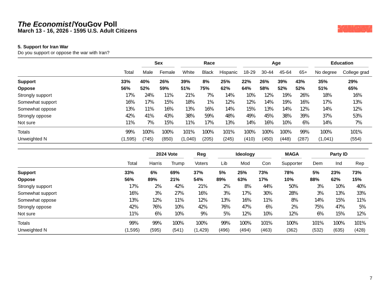
In the AI era, we might be tempted to ask an LLM to extract the data for us. But should you?

Using LLMs to extract unstructured data from PDFs requires careful prompting and expensive API calls (or monthly plan), and the results may be unreliable. Instead, we can just write code to do it in R!

Extracting tables with {tabulapdf}

The {tabulapdf} package wraps the Java Tabula library to extract tables from PDFs:

library(tabulapdf)

iran_war <- extract_tables(
  file = "data/econTabReport_CwWXhS2.pdf",
  pages = 7,
  col_names = FALSE
) |>
  pluck(1)

1

pages = 7 extracts tables from page 7 only.

2

col_names = FALSE prevents the first row from being treated as column names — the raw table has merged headers that require manual cleaning.

3

pluck(1) extracts the first (and only) table from the list returned by extract_tables().

# A tibble: 22 × 11
   X1               X2    X3    X4           X5    X6    X7        X8    X9    X10   X11  
   <chr>            <chr> <chr> <chr>        <chr> <chr> <chr>     <lgl> <chr> <lgl> <chr>
 1 <NA>             <NA>  <NA>  Sex          <NA>  Race  <NA>      NA    Age   NA    Educ…
 2 <NA>             Total Male  Female White <NA>  Black Hispanic… NA    30-4… NA    No d…
 3 Support          33%   40%   26% 39%      <NA>  8%    25% 22%   NA    26% … NA    35% …
 4 Oppose           56%   52%   59% 51%      <NA>  75%   62% 64%   NA    58% … NA    51% …
 5 Strongly support 17%   24%   11%          21%   7%    14% 10%   NA    12% … NA    18% …
 6 Somewhat support 16%   17%   15%          18%   1%    12% 12%   NA    14% … NA    17% …
 7 Somewhat oppose  13%   11%   16%          13%   16%   14% 15%   NA    13% … NA    14% …
 8 Strongly oppose  42%   41%   43%          38%   59%   48% 49%   NA    45% … NA    37% …
 9 Not sure         11%   7%    15%          11%   17%   13% 14%   NA    16% … NA    14% …
10 Totals           99%   100%  100% 101%    <NA>  100%  101% 100% NA    100%… NA    100%…
# ℹ 12 more rows

Cleaning and tidying

The raw extracted table has all columns concatenated in odd ways. Manual inspection of the rows and columns reveals which contain the relevant data:

iran_war |>
  slice(16:20) |>
  select(X1, X11) |>

  separate_wider_delim(
    cols = X11,
    delim = " ",
    names = c("Democrats", "Independents", "Republicans")
  ) |>
  rename(response = X1)

1

Rows 16–20 contain the five response options (Strongly support through Strongly oppose). Other rows contain headers and totals.

2

X1 holds the response label; X11 holds the three party percentages concatenated with spaces.

3

separate_wider_delim() splits the concatenated party column into three separate columns on the space delimiter.

# A tibble: 5 × 4
  response         Democrats Independents Republicans
  <chr>            <chr>     <chr>        <chr>      
1 Strongly support 3%        10%          40%        
2 Somewhat support 3%        13%          33%        
3 Somewhat oppose  14%       15%          11%        
4 Strongly oppose  75%       47%          5%         
5 Not sure         6%        15%          12%        

Visualizing Likert scale data

A Likert scale is a symmetric rating scale with a neutral midpoint, typically used to measure attitudes or opinions:

1. Strongly disagree
2. Somewhat disagree
3. Neither agree nor disagree
4. Somewhat agree
5. Strongly agree

Likert responses are ordered but not continuous. This ordering, and the fact that responses split on both sides of the neutral midpoint, creates the main design challenge.

Design 1: Stacked bar charts

The simplest approach stacks all responses from left to right in a single bar per group:

iran_war_long <- iran_war |>
  slice(16:20) |>
  select(X1, X11) |>
  separate_wider_delim(
    cols = X11,
    delim = " ",
    names = c("Democrats", "Independents", "Republicans")
  ) |>
  rename(response = X1) |>
  pivot_longer(
    cols = -response,
    names_to = "pid3",
    values_to = "pct",
    values_transform = \(x) parse_number(x) / 100
  ) |>
  mutate(
    response = factor(
      response,
      levels = c(
        "Strongly support",
        "Somewhat support",
        "Not sure",
        "Somewhat oppose",
        "Strongly oppose"
      )
    ),
    pid3 = factor(pid3, levels = c("Democrats", "Independents", "Republicans"))
  ) |>
  mutate(pct = pct / sum(pct), .by = pid3)

stack_bar_p <- ggplot(
  data = iran_war_long,
  mapping = aes(x = pct, y = pid3, fill = response)
) +
  geom_col() +
  scale_x_continuous(labels = label_percent(), position = "top") +
  scale_fill_discrete_diverging(
    palette = "Blue-Red",
    labels = label_wrap(width = 8),
    guide = guide_legend(
      reverse = TRUE,
      theme = theme(legend.key.width = unit(1, "cm"))
    )
  ) +
  labs(
    x = NULL,
    y = NULL,
    fill = NULL,
    title = "Do you support or oppose the war with Iran?",
    caption = "Source: YouGov (March 13–16, 2026)"
  ) +
  theme(
    legend.position = "bottom",
    panel.grid = element_blank(),
    axis.ticks.y = element_blank(),
    axis.ticks.length.x = unit(0.25, "cm")
  )
stack_bar_p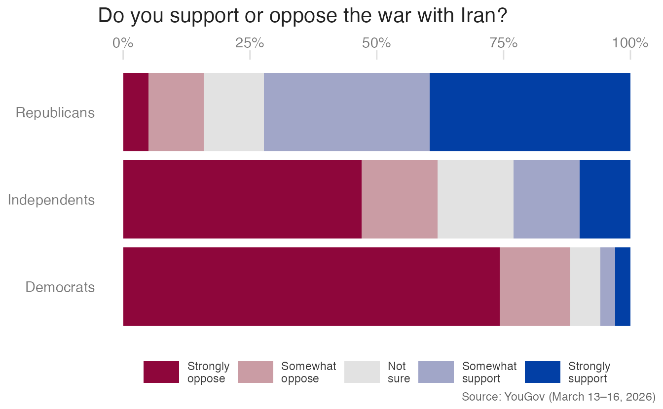

• Advantage: Straightforward to produce; readers can judge total support vs. total opposition for each party.
• Limitation: The neutral midpoint is not aligned across groups, making it hard to compare intensities (e.g., “Strongly support” proportions across parties).

A minor variant on this approach adds a mirrored axis on the bottom (showing proportions from right to left) lets readers read opposition from either end:

stack_bar_p +
  scale_x_continuous(
    labels = label_percent(),
    position = "top",
    sec.axis = sec_axis(
      transform = \(x) 1 - x,
      labels = label_percent(),
      name = NULL
    )
  )

1

sec_axis() adds a secondary axis. transform = \(x) 1 - x converts the primary scale (0–100% from the left) to a mirrored scale (0–100% from the right), allowing readers to read opposition from either edge.

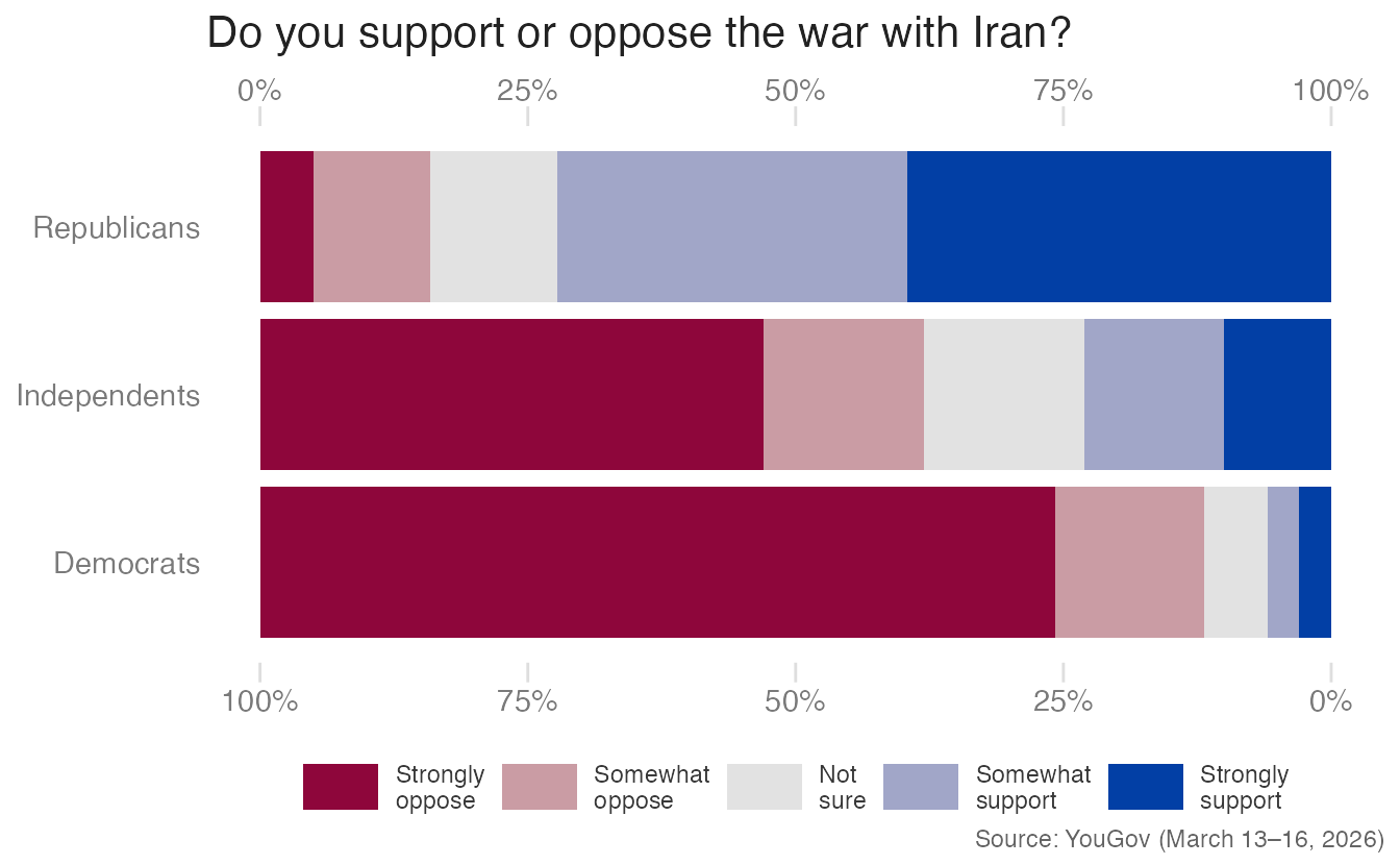
• Advantage: Makes both support and opposition directly readable without arithmetic.
• Limitation: The neutral/unsure responses remain embedded in the bar, obscuring their size.

Design 2: Diverging bars, neutrals separate

Placing oppose responses to the left and support responses to the right of a zero origin creates a diverging chart. Neutral responses are separated into their own panel to avoid mixing them with the diverging logic:

div_bar_no_neutral_p <- iran_war_long |>
  filter(response != "Not sure") |>
  mutate(
    pct = if_else(
      response %in% c("Strongly oppose", "Somewhat oppose"),
      -pct,
      pct
    ),
    response = as.character(response)
  ) |>
  ggplot(mapping = aes(x = pct, y = pid3, fill = response)) +
  geom_col(position = position_stack(reverse = TRUE)) +
  scale_x_continuous(
    breaks = seq(from = -.8, to = .6, by = .2),
    labels = label_percent(),
    position = "top"
  ) +
  scale_fill_manual(
    labels = label_wrap(width = 8),
    breaks = c(
      "Strongly support",
      "Somewhat support",
      "Not sure",
      "Somewhat oppose",
      "Strongly oppose"
    ),
    values = diverging_hcl(palette = "Blue-Red", n = 5),
    guide = guide_legend(
      reverse = TRUE,
      theme = theme(legend.key.width = unit(1, "cm"))
    )
  ) +
  labs(x = NULL, y = NULL, fill = NULL) +
  theme(
    legend.position = "bottom",
    panel.grid = element_blank(),
    axis.ticks.y = element_blank(),
    axis.ticks.length.x = unit(0.25, "cm")
  )

div_bar_neutral_p <- iran_war_long |>
  filter(response == "Not sure") |>
  ggplot(mapping = aes(x = pct, y = pid3, fill = response)) +
  geom_col(position = position_stack(reverse = TRUE)) +
  scale_x_continuous(
    breaks = c(0, .2),
    limits = c(NA, .2),
    labels = label_percent(),
    position = "top"
  ) +
  scale_fill_discrete_diverging(
    palette = "Blue-Red",
    labels = label_wrap(width = 8),
    guide = guide_legend(
      reverse = TRUE,
      theme = theme(legend.key.width = unit(1, "cm"))
    )
  ) +
  labs(x = NULL, y = NULL, fill = NULL) +
  theme(
    legend.position = "bottom",
    panel.grid = element_blank(),
    axis.ticks.y = element_blank(),
    axis.ticks.length.x = unit(0.25, "cm")
  )

div_bar_no_neutral_p +
  div_bar_neutral_p +
  plot_annotation(
    title = "Do you support or oppose the war with Iran?",
    caption = "Source: YouGov (March 13–16, 2026)"
  ) +
  plot_layout(widths = c(4, 1), axes = "collect")

1

The response variable must be converted to a character vector before manual fill assignment, since scale_fill_manual() with breaks may mis-order factor levels.

2

diverging_hcl(palette = "Blue-Red", n = 5) generates five colors from the {colorspace} diverging palette, matching them manually to the five response levels.

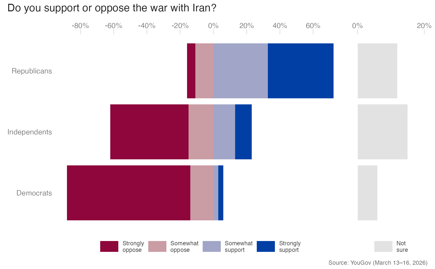
• Advantage: The neutral/unsure bar is clearly separated and its size is easy to read.
• Limitation: Two panels require side-by-side layout with shared y-axis, which adds production complexity.

Design 3: Diverging bars, neutrals integrated

An alternative places neutral responses symmetrically: half extends left, half extends right. This keeps all responses in a single panel while still centering at zero:

iran_war_long |>
  mutate(pct_plot = if_else(response == "Not sure", pct / 2, pct)) |>
  uncount(
    weights = if_else(response == "Not sure", 2L, 1L),
    .id = "neutral_half"
  ) |>
  mutate(
    pct_plot = case_when(
      response %in% c("Strongly oppose", "Somewhat oppose") ~ -pct_plot,
      response == "Not sure" & neutral_half == 1L ~ -pct_plot,
      .default = pct_plot
    ),
    response = as.character(response)
  ) |>
  ggplot(mapping = aes(x = pct_plot, y = pid3, fill = response)) +
  geom_col(position = position_stack(reverse = TRUE)) +
  geom_vline(xintercept = 0, linewidth = 0.4, color = "gray40") +
  scale_x_continuous(
    breaks = seq(from = -.8, to = .6, by = .2),
    labels = label_percent(),
    position = "top"
  ) +
  scale_fill_manual(
    labels = label_wrap(width = 8),
    breaks = c(
      "Strongly support",
      "Somewhat support",
      "Not sure",
      "Somewhat oppose",
      "Strongly oppose"
    ),
    values = diverging_hcl(palette = "Blue-Red", n = 5),
    guide = guide_legend(
      reverse = TRUE,
      theme = theme(legend.key.width = unit(1, "cm"))
    )
  ) +
  labs(
    x = NULL,
    y = NULL,
    fill = NULL,
    title = "Do you support or oppose the war with Iran?",
    caption = "Source: YouGov (March 13–16, 2026)"
  ) +
  theme(
    legend.position = "bottom",
    panel.grid = element_blank(),
    axis.ticks.y = element_blank(),
    axis.ticks.length.x = unit(0.25, "cm")
  )

1

The neutral proportion is halved before duplication.

2

uncount() duplicates neutral rows twice (once for each half), adding a neutral_half index column.

3

One neutral half is inverted to negative, placing it on the left of zero; the other stays positive.

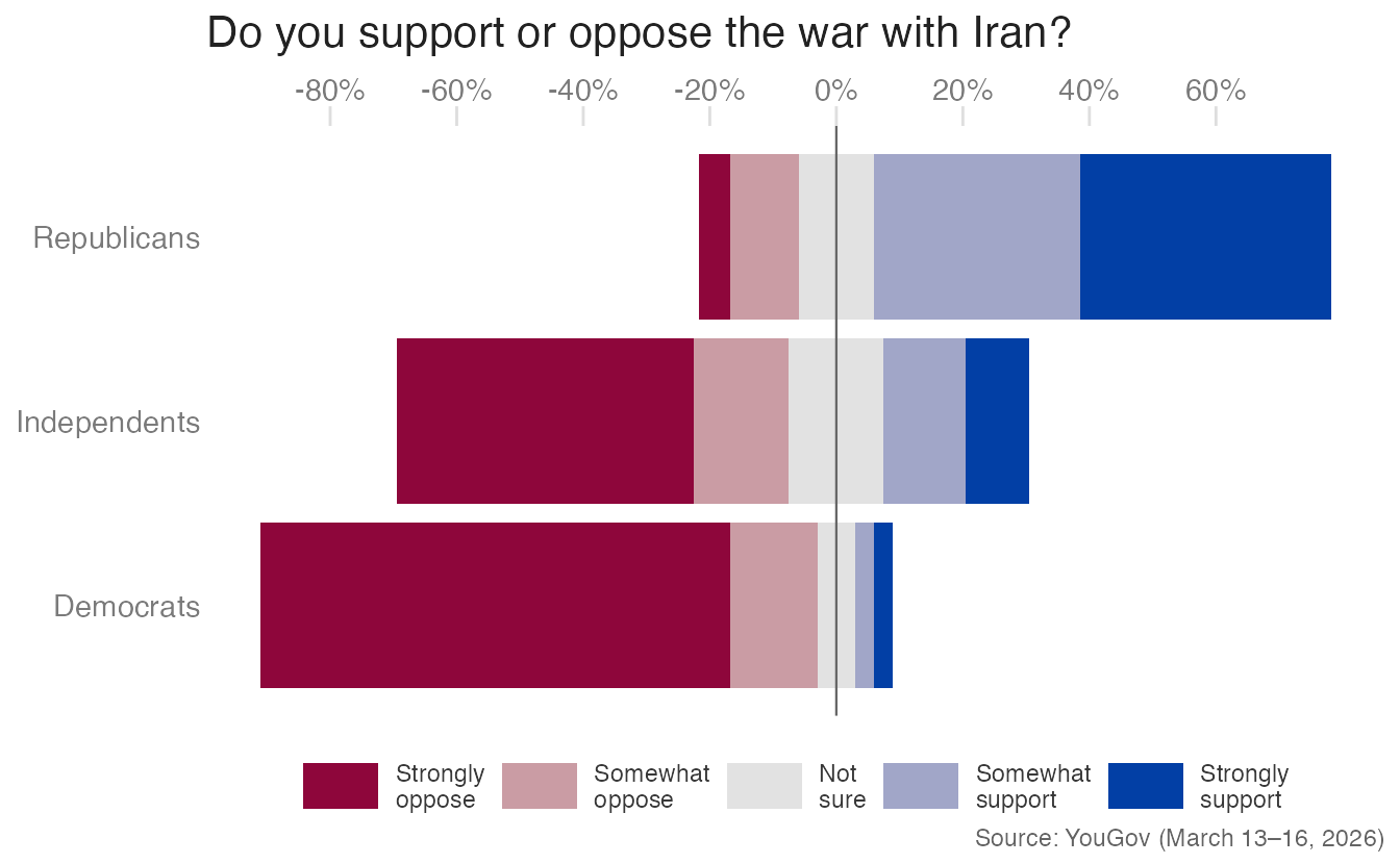
• Advantage: Single-panel layout; symmetric diverging structure with the neutral midpoint visible.
• Limitation: The neutral/unsure portion is harder to read precisely because it is split across the center line.

Design 4: Split bars (small multiples)

Faceting by response option creates one bar per response category, making individual category comparisons across parties very easy:

ggplot(
  data = iran_war_long,
  mapping = aes(x = pct, y = pid3, fill = response)
) +
  geom_col() +
  scale_x_continuous(
    breaks = seq(from = 0, to = 1, by = 0.2),
    labels = label_percent(),
    position = "top"
  ) +
  scale_fill_discrete_diverging(palette = "Blue-Red", guide = "none") +
  facet_wrap(
    facets = vars(response |> fct_rev()),
    nrow = 1,
    space = "free_x",
    scales = "free_x",
    labeller = label_wrap_gen(width = 15)
  ) +
  labs(
    x = NULL,
    y = NULL,
    fill = NULL,
    title = "Do you support or oppose the war with Iran?",
    caption = "Source: YouGov (March 13–16, 2026)"
  ) +
  theme(
    panel.grid = element_blank(),
    axis.ticks.y = element_blank(),
    axis.ticks.length.x = unit(0.25, "cm"),
    strip.text = element_text(
      size = rel(0.7),
      margin = margin(t = 1, r = 0, b = 1, l = 0, unit = "mm")
    )
  )

1

space = "free_x" with scales = "free_x" makes each panel’s axis range match its data. This means “Strongly support” and “Strongly oppose” panels use a narrower axis than “Somewhat support”, preventing small values from appearing artificially large.

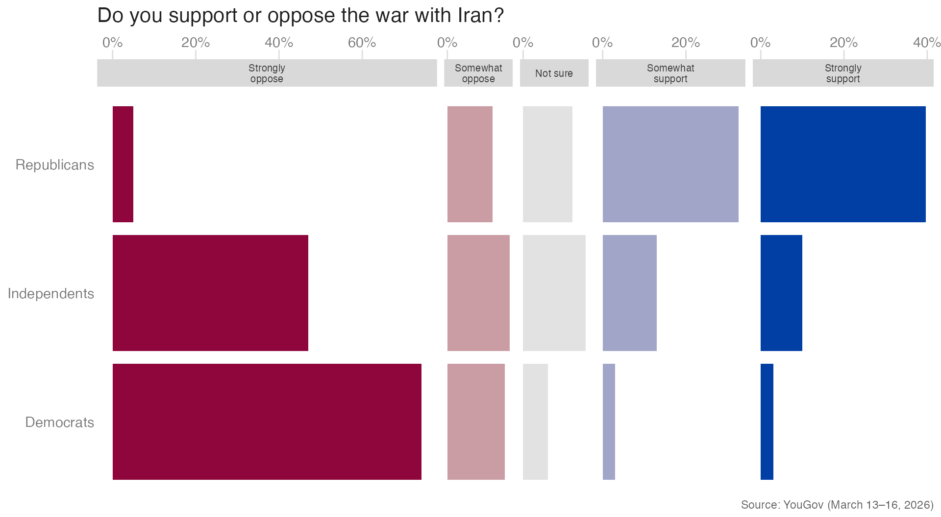
• Advantage: The clearest design for comparing a single response option across groups; there is no stacking confusion.
• Limitation: It is harder to assess the overall distribution (how much total support vs. opposition) within a single group, since you have to look across panels.

Choosing a design

We have seen four primary methods for constructing diverging bar charts for survey data.

1. Stacked bar charts: all responses are plotted in a single bar, with negative responses on the left and positive responses on the right. Neutral responses are included in the middle of the bar.
2. Diverging, with extra neutrals: negative and positive responses are plotted in separate bars on either side of the origin, with neutral responses in a distinct, separate subplot.
3. Diverging, integrated neutrals: negative and positive responses are plotted in separate bars on either side of the origin, but neutral responses are centered around the origin.
4. Split bars: each response category is plotted in a separate facet, with negative responses on the left and positive responses on the right. Neutral responses are plotted in their own facet in the middle.

(a) Stacked bar charts

(b) Diverging, with extra neutrals

(c) Diverging, integrated neutrals

(d) Split bars

Figure 1: An example of each of the four methods for plotting diverging bar charts for survey data.

Your turn: Evaluate each of the four methods for plotting diverging bar charts, specifically identifying how it enables (or does not) specific tasks.

	Stacked bar charts	Diverging, with extra neutrals	Diverging, integrated neutrals	Split bars	How important do we think it is?
Read percentage of values of     and
Read percentage of values of
Read percentage of values of
Read percentage of values of
Read percentage of values of
Read percentage of values of
Read percentage of values of     and

NoteSuggested solution

	Stacked bar charts	Diverging, with extra neutrals	Diverging, integrated neutrals	Split bars	How important do we think it is?
Read percentage of values of     and	👍	👍	👎	👎	Very important
Read percentage of values of	👍	👎	👎	👍	Important
Read percentage of values of	👎	👍	👎	👍	Important
Read percentage of values of	👎	👍	👎	👍	Not important
Read percentage of values of	👎	👍	👎	👍	Important
Read percentage of values of	👍 (with double axis)	👎	👎	👍	Important
Read percentage of values of     and	👍 (with double axis)	👍	👎	👎	Very important

Summary

• Survey data is often distributed as Stata or SPSS files; use {haven}’s read_dta() / read_sav() to import, then as_factor() to convert labeled variables
• Survey weights correct for sampling imbalances; use the {srvyr} package to compute weighted proportions and means with as_survey_design() + survey_mean()
• Top-line PDFs can be parsed programmatically with {tabulapdf}’s extract_tables(); expect manual cleaning of column structure
• For Likert data, the choice between stacked, diverging (with separate neutrals), diverging (with integrated neutrals), and split bar designs depends on what comparison you want to enable
• Use a diverging color palette (scale_fill_discrete_diverging()) to encode the agree/disagree dimension

Acknowledgements

Diverging bar charts examples drawn from The case against diverging stacked bars by Lisa Charlotte Muth and Gregor Aisch. Material derived in part from STA 313: Advanced Data Visualization.