Interactive reporting with Shiny I

ImportantGetting started

• Go to the course GitHub org and find your ae-shiny (repo name will be suffixed with your GitHub name).
• Clone the repo in Positron, follow along, and complete the exercises embedded throughout the notes.

NoteLearning objectives

• Introduce Shiny for interactive web applications
• Review implementation of a basic Shiny app
• Introduce reactive programming concepts

What is Shiny?

Shiny is a web application framework for R (and Python!) that allows you to build interactive web applications using R code. A Shiny app is a live, running R process: when a reader changes an input (selects a dropdown, moves a slider), the server re-executes R code and sends the updated output back to the browser.

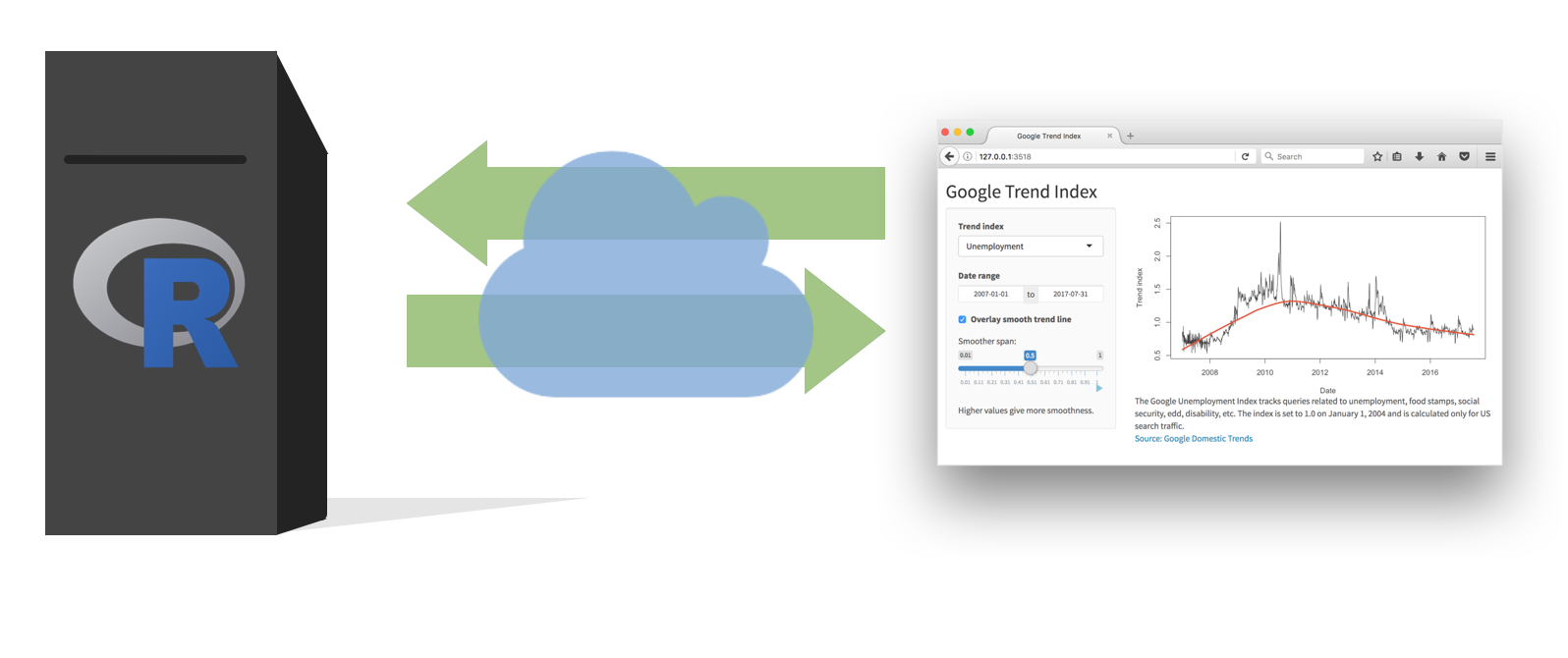
Because the R process is always running, Shiny apps can do anything R can do: query databases, fit models, process uploaded files, and regenerate any output in response to any input. The tradeoff is that you need a server to host a Shiny app.

How Shiny works

When running locally, the computer serving the app is your own machine.

When deployed, the computer serving the app is a remote web server.

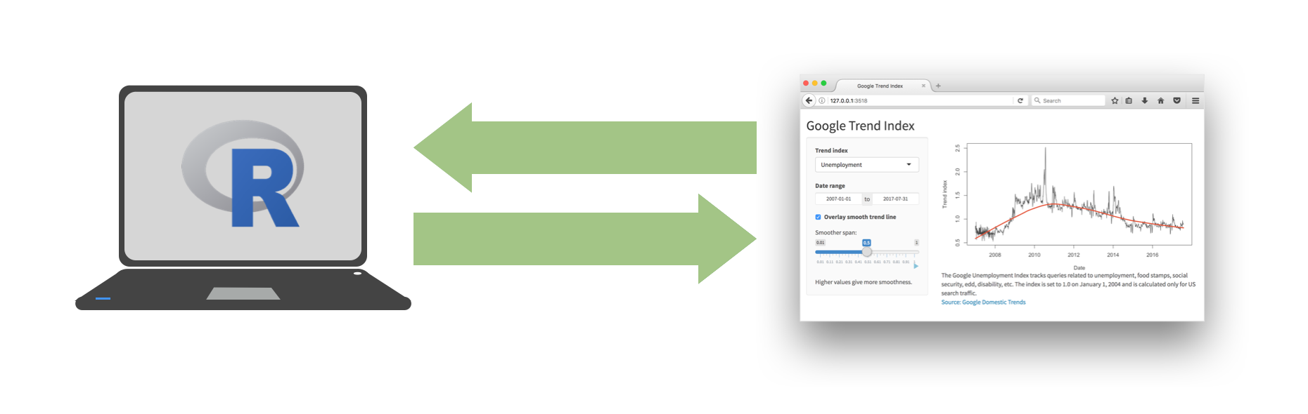
The key insight is that the browser is just a display layer. The computations happen in R on the server, and only the rendered output (HTML, images, tables) is sent to the browser.

Dating rules

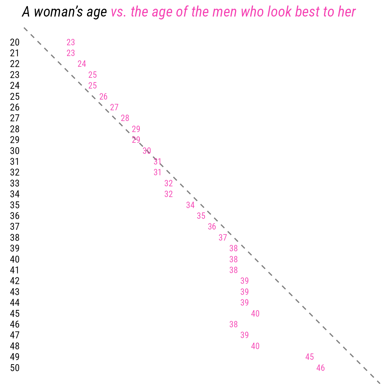
There are many attitudes and trends surrounding age gaps in sexual relationships. Based on research by Christian Rudder, founder of OKCupid, women tend to prefer men around their own age.

Figure 1: Source: Christian Rudder, Dataclysm.

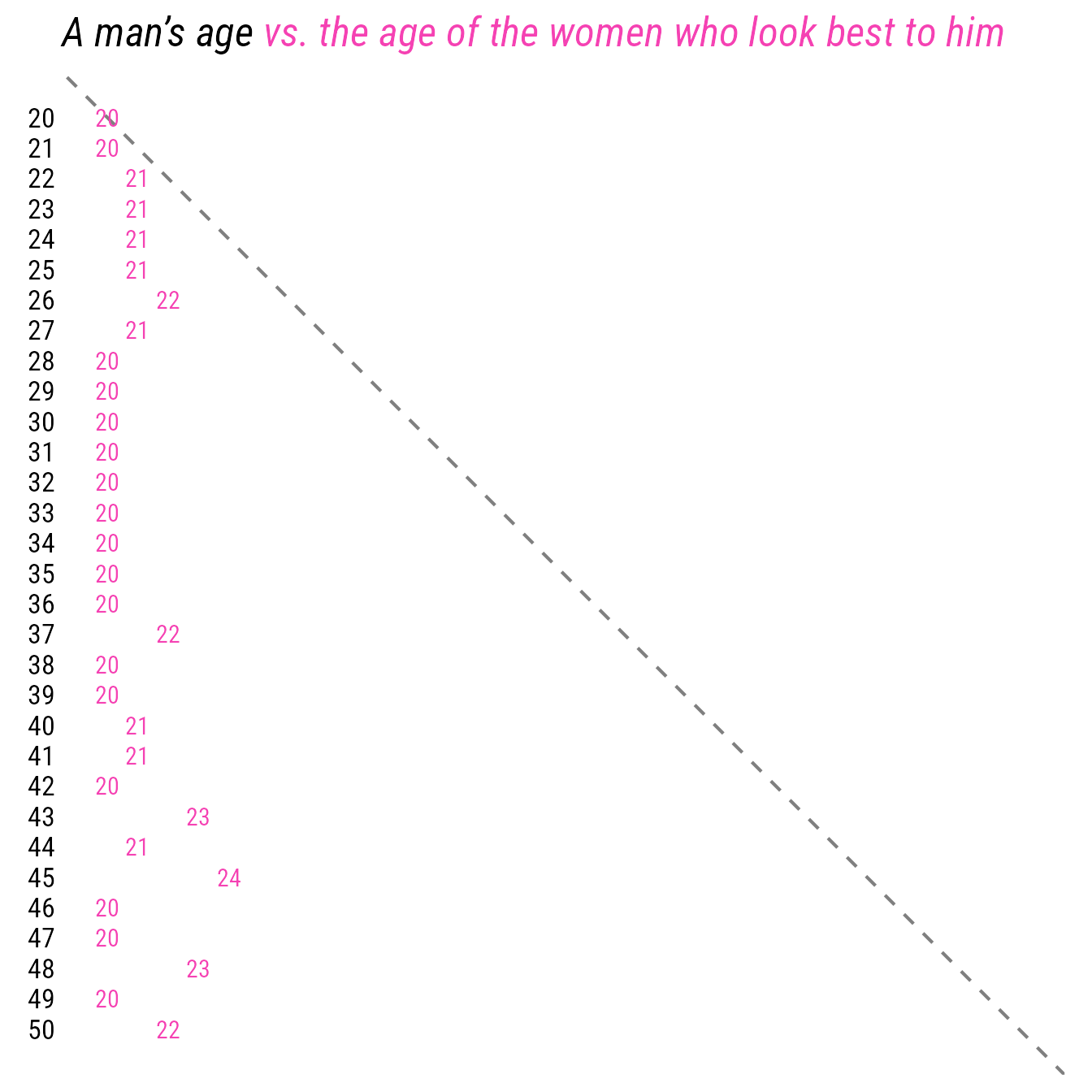
Men, however, tend to adhere to the Leonardo DiCaprio rule:

Figure 2: Source: Christian Rudder, Dataclysm.

For those whom are concerned with the ethics of age gaps in relationships, the “half your age plus seven” rule is a common heuristic for determining socially acceptable age differences. The rule states that the youngest person you should date is half your age plus seven years.

Some may find the arithmetic of this rule to be a bit tedious, so I built a Shiny app to make it easier to apply. Take note of the different interactive components of the app and how they work together to generate the output.

Anatomy of a Shiny app

Every Shiny app has exactly two components:

library(shiny)
library(bslib)

ui <- list()

server <- function(input, output, session) {}

shinyApp(ui = ui, server = server)

1

The UI (user interface) defines how the app looks: layouts, input widgets, and output placeholders.

2

The server function contains the reactive logic that generates outputs from inputs.

3

shinyApp() links the UI and server and launches the app.

This structure is the same for apps of any complexity — from a single slider to a multi-page dashboard.

{shiny} and {bslib}

library(shiny)
library(bslib)

library(shiny) + library(bslib) is now the officially recommended way to build Shiny apps. {bslib} provides a modern UI toolkit based on Bootstrap, with cleaner layout functions and better theming support.

NoteStylistic differences between {shiny} and {bslib}

{shiny} functions use camelCase (e.g., plotOutput(), renderPlot()), while {bslib} functions use snake_case (e.g., page_sidebar(), value_box()). This distinction helps identify which package a function comes from.

A first app

The best way to understand Shiny is to build one. Throughout this unit, we will use a weather dataset which contains daily observations from US airports:

d <- read_csv("data/weather.csv")

glimpse(d)

Rows: 23,376
Columns: 17
$ id             <dbl> 72202, 72202, 72202, 72202, 72202, 72202, 72202, 72202, 72202, 72…
$ name           <chr> "Miami", "Miami", "Miami", "Miami", "Miami", "Miami", "Miami", "M…
$ airport_code   <chr> "KMIA", "KMIA", "KMIA", "KMIA", "KMIA", "KMIA", "KMIA", "KMIA", "…
$ country        <chr> "US", "US", "US", "US", "US", "US", "US", "US", "US", "US", "US",…
$ state          <chr> "FL", "FL", "FL", "FL", "FL", "FL", "FL", "FL", "FL", "FL", "FL",…
$ region         <chr> "South", "South", "South", "South", "South", "South", "South", "S…
$ longitude      <dbl> -80.3167, -80.3167, -80.3167, -80.3167, -80.3167, -80.3167, -80.3…
$ latitude       <dbl> 25.7833, 25.7833, 25.7833, 25.7833, 25.7833, 25.7833, 25.7833, 25…
$ date           <date> 2022-01-01, 2022-01-02, 2022-01-03, 2022-01-04, 2022-01-05, 2022…
$ temp_avg       <dbl> 24.2, 24.4, 22.7, 20.4, 22.9, 21.4, 23.6, 23.9, 23.8, 24.0, 21.4,…
$ temp_min       <dbl> 21.1, 21.7, 17.8, 16.7, 19.4, 16.7, 20.6, 22.2, 22.2, 21.1, 18.3,…
$ temp_max       <dbl> 27.8, 28.3, 27.2, 25.6, 27.2, 26.7, 28.3, 26.1, 26.1, 27.8, 25.0,…
$ precip         <dbl> 0.0, 0.0, 0.0, 0.0, 5.3, 0.0, 0.0, 4.3, 4.6, 0.0, 23.9, 0.3, 0.3,…
$ snow           <dbl> 0, 0, 0, 0, 0, 0, 0, 0, 0, 0, 0, 0, 0, 0, 0, 0, 0, 0, 0, 0, 0, 0,…
$ wind_direction <dbl> 130, 164, 261, 27, 142, 330, 5, 58, 87, 53, 5, 58, 328, 319, 75, …
$ wind_speed     <dbl> 12.2, 12.6, 10.8, 10.8, 9.4, 5.0, 7.6, 16.9, 21.6, 6.5, 13.3, 15.…
$ air_press      <dbl> 1018.6, 1018.0, 1018.7, 1019.8, 1015.9, 1016.5, 1019.1, 1024.5, 1…

Here is a minimal app that lets the reader choose an airport and displays a temperature time series:

demos/demo-01.R

library(tidyverse)
library(shiny)
library(bslib)

d <- read_csv("data/weather.csv")


ui <- page_sidebar(
  title = "Temperatures at Major Airports",

  sidebar = sidebar(
    radioButtons(
      inputId = "name",
      label = "Select an airport",
      choices = c(
        "Hartsfield-Jackson Atlanta",
        "Raleigh-Durham",
        "Denver",
        "Los Angeles",
        "John F. Kennedy"
      )
    )
  ),
  plotOutput(outputId = "plot")
)

server <- function(input, output, session) {

  output$plot <- renderPlot({
    d |>
      filter(name %in% input$name) |>
      ggplot(mapping = aes(x = date, y = temp_avg)) +
      geom_line()
  })
}

shinyApp(ui = ui, server = server)

1

page_sidebar() from {bslib} creates a two-pane layout with a sidebar on the left and a main body on the right.

2

sidebar() wraps the input widgets that appear in the left panel.

3

inputId = "name" is the ID used to retrieve this input’s current value in the server.

4

plotOutput(outputId = "plot") reserves space in the UI for a plot; it starts empty.

5

renderPlot({...}) in the server generates the plot and assigns it to output$plot, which fills the placeholder in the UI.

6

input$name accesses the current value of the "name" radio button — it is reactive: the plot re-renders automatically whenever the selection changes.

Note⌨️ Your turn

Open exercises/ex-01.R and execute it via the Run App button.

Check that you are able to successfully run the Shiny app and are able to interact with it by picking a new airport.

If everything is working, try modifying the code:

• Try adding or removing a city from radioButtons()
• Check what happens if you add a city that is not in weather.csv (i.e. Ithaca)

You can use unique(d$name) to see the list of available airports in the data.

UI layouts

Page layout functions

Shiny uses page layout functions to specify the overall structure of the UI. page_sidebar() is a good default for simple apps: a title, a sidebar (usually holding inputs), and a main body (usually holding outputs).

Other common layouts include:

• page_fluid() — a flexible multi-row layout
• page_navbar() — adds a navigation bar with multiple tab pages
• page_fillable() — content fills the available viewport height

See the full layout gallery at https://shiny.posit.co/r/layouts/.

Shiny vs {bslib} layouts

If you have seen older Shiny code, you may have seen fluidPage() + sidebarLayout() — these are {shiny}’s original layout functions. {bslib} provides modern equivalents (page_sidebar(), page_fluid()) with cleaner syntax. Both work; {bslib} is preferred for new apps.

UI functions generate HTML

Shiny UI functions are R functions that return HTML. Run any of the following in the R console to see the underlying HTML:

actionButton("id", "Click me!")
selectInput("test", "Test", choices = c("A", "B", "C"), selectize = FALSE)
img(src = "shiny.png")

<button id="id" type="button" class="btn btn-default action-button"><span class="action-label">Click me!</span></button>

<div class="form-group shiny-input-container">
  <label class="control-label" id="test-label" for="test">Test</label>
  <div>
    <select class="shiny-input-select form-control" id="test"><option value="A" selected>A</option>
<option value="B">B</option>
<option value="C">C</option></select>
  </div>
</div>

<img src="shiny.png"/>

This means you can generate UI dynamically using standard R code — helpful when building inputs whose choices depend on the data.

Inputs

Input widgets collect user selections and make them available in the server as input$<inputId>. A few key inputs:

radioButtons(
  inputId = "name",
  label = "Select an airport",
  choices = c("Denver", "Los Angeles", "JFK")
)

selectInput(
  inputId = "var",
  label = "Select a variable",
  choices = c("Average temp" = "temp_avg", "Max temp" = "temp_max"),
  selected = "temp_avg"
)

sliderInput(
  inputId = "num",
  label = "Choose a number",
  min = 0,
  max = 100,
  value = 20
)

1

radioButtons() — one selection from a set of options, displayed as a list.

2

selectInput() — a dropdown; set multiple = TRUE to allow multi-select. The vector can have "Display name" = "column_name" form to show a friendly label.

3

sliderInput() — a draggable range slider.

All input widgets follow the same pattern: inputId, label, and widget-specific arguments. The full gallery is embedded below and at https://shiny.posit.co/r/components/#inputs.

Note⌨️ Your turn

Starting from the code in exercises/ex-02.R try changing the radioButton() input to one of the following:

• selectInput() with multiple = FALSE

• selectInput() with multiple = TRUE

• checkboxGroupInput()

What happens? Does the app still work as expected?

Outputs

Output functions reserve space in the UI for rendered content. They come in matched pairs: one function in the UI, one in the server.

UI function	Server function	Content
plotOutput()	renderPlot({})	A {ggplot2} or base R plot
tableOutput()	renderTable({})	An R data frame as an HTML table
uiOutput()	renderUI({})	Dynamically generated UI elements
textOutput()	renderText({})	A character string

The outputId in the UI must match the name used in output$<name> in the server. The full gallery is embedded below and at https://shiny.posit.co/r/components/#outputs.

Basic reactivity

The reactive graph

Shiny applications are driven by reactive programming: outputs automatically re-execute whenever the inputs they depend on change. The dependency relationships form a reactive graph.

For the first demo app:

When the reader changes the name radio button, Shiny detects that input$name is used inside output$plot’s renderPlot({}) expression, and re-executes just that expression.

Adding a second input

Extending the app to let the reader also choose which weather variable to plot adds a second node to the reactive graph:

demos/demo-02.R

d_vars <- c(
  "Average temp" = "temp_avg",
  "Min temp" = "temp_min",
  "Max temp" = "temp_max",
  "Total precip" = "precip",
  "Wind speed" = "wind_speed"
)

ui <- page_sidebar(
  title = "Weather Forecasts",
  sidebar = sidebar(
    radioButtons(
      inputId = "name",
      label = "Select an airport",
      choices = c("Raleigh-Durham", "Denver", "Los Angeles", "JFK")
    ),
    selectInput(
      inputId = "var",
      label = "Select a variable",
      choices = d_vars,
      selected = "temp_avg"
    )
  ),
  plotOutput(outputId = "plot")
)

server <- function(input, output, session) {
  output$plot <- renderPlot({
    d |>
      filter(name %in% input$name) |>
      ggplot(mapping = aes(x = date, y = .data[[input$var]])) +
      geom_line() +
      labs(title = str_c(input$name, " - ", input$var))
  })
}

shinyApp(ui = ui, server = server)

1

.data[[input$var]] uses the .data pronoun from {rlang} to reference a data frame column by a variable name stored as a string. This is the idiomatic way to use reactive column names in {tidyverse} pipelines — it avoids the complexity of !!, enquo(), and other tidy evaluation tools.

The reactive graph now has two inputs feeding one output:

Both input$name and input$var are detected as dependencies of output$plot, so any change to either triggers a re-render.

Note⌨️ Your turn

Starting with the code in exercises/ex-03.R (based on demo-02.R’s code) add a tableOutput() with the id minmax to the app’s body.

Once you have done that, you should then add logic to the server() function to render the table so that it shows the min and max average temperature for each year contained in the data.

• You will need to add an appropriate output in the ui
• And a corresponding reactive expression in the server() function to generate these summaries.
• lubridate::year() will be useful along with dplyr::summarize().

Summary

• A Shiny app has two components — a UI that defines appearance and an input/output layout, and a server function that contains reactive logic
• {bslib} provides modern layout functions (page_sidebar(), page_fluid()) that replace the older {shiny} layout functions
• Input widgets (radioButtons(), selectInput(), sliderInput()) collect reader selections and expose them as input$<id> in the server
• Output functions come in matched UI/server pairs: plotOutput() / renderPlot({}), tableOutput() / renderTable({}), etc.
• Shiny automatically detects which outputs depend on which inputs and re-executes only the necessary render functions when an input changes

Acknowledgements

Material derived in part from posit::conf 2025 - Shiny for R Workshop by Colin Rundel (CC BY 4.0) and Advanced Data Visualization.