Data wrangling (I)

NoteLearning objectives

• Identify the importance of data wrangling for effective data communication
• Demonstrate common data transformation operations with {dplyr}
• Explain the principles of tidy data
• Reshape data from wide to long format using pivot_longer()

Data: Penguins

We’ll use the penguins dataset throughout this lesson to demonstrate {dplyr} operations. If you need a reminder of its structure:

glimpse(penguins)

Rows: 344
Columns: 8
$ species     <fct> Adelie, Adelie, Adelie, Adelie, Adelie, Adelie, Adelie, Adelie, Adel…
$ island      <fct> Torgersen, Torgersen, Torgersen, Torgersen, Torgersen, Torgersen, To…
$ bill_len    <dbl> 39.1, 39.5, 40.3, NA, 36.7, 39.3, 38.9, 39.2, 34.1, 42.0, 37.8, 37.8…
$ bill_dep    <dbl> 18.7, 17.4, 18.0, NA, 19.3, 20.6, 17.8, 19.6, 18.1, 20.2, 17.1, 17.3…
$ flipper_len <int> 181, 186, 195, NA, 193, 190, 181, 195, 193, 190, 186, 180, 182, 191,…
$ body_mass   <int> 3750, 3800, 3250, NA, 3450, 3650, 3625, 4675, 3475, 4250, 3300, 3700…
$ sex         <fct> male, female, female, NA, female, male, female, male, NA, NA, NA, NA…
$ year        <int> 2007, 2007, 2007, 2007, 2007, 2007, 2007, 2007, 2007, 2007, 2007, 20…

Data wrangling with {dplyr}

Raw data rarely arrives in the exact form a visualization needs. Variable types are wrong, irrelevant columns clutter the frame, values need to be recoded, and summaries need to be computed. Data wrangling is the process of transforming raw data into a form suitable for visualization or analysis.

{dplyr} provides a consistent set of verbs for the most common transformations. Each function takes a data frame as its first argument and returns a data frame — this makes them easy to chain together with the pipe (|>).

NoteR for Data Science

This is a brief introduction to data wrangling with {dplyr}. For a more comprehensive treatment, see R for Data Science.

Filtering rows

filter() keeps rows that satisfy a condition. The condition is written as a logical expression:

penguins |>
  filter(species == "Chinstrap")

1

Keep only Chinstrap penguins. == tests for equality; use != for not-equal, >, <, >=, <= for comparisons, and & / | for AND / OR.

# A tibble: 68 × 8
   species   island bill_len bill_dep flipper_len body_mass sex     year
   <fct>     <fct>     <dbl>    <dbl>       <int>     <int> <fct>  <int>
 1 Chinstrap Dream      46.5     17.9         192      3500 female  2007
 2 Chinstrap Dream      50       19.5         196      3900 male    2007
 3 Chinstrap Dream      51.3     19.2         193      3650 male    2007
 4 Chinstrap Dream      45.4     18.7         188      3525 female  2007
 5 Chinstrap Dream      52.7     19.8         197      3725 male    2007
 6 Chinstrap Dream      45.2     17.8         198      3950 female  2007
 7 Chinstrap Dream      46.1     18.2         178      3250 female  2007
 8 Chinstrap Dream      51.3     18.2         197      3750 male    2007
 9 Chinstrap Dream      46       18.9         195      4150 female  2007
10 Chinstrap Dream      51.3     19.9         198      3700 male    2007
# ℹ 58 more rows

Multiple conditions can be combined in a single filter() call:

penguins |>
  filter(species == "Adelie", island == "Dream")

1

Comma-separated conditions are combined with AND — both must be true.

# A tibble: 56 × 8
   species island bill_len bill_dep flipper_len body_mass sex     year
   <fct>   <fct>     <dbl>    <dbl>       <int>     <int> <fct>  <int>
 1 Adelie  Dream      39.5     16.7         178      3250 female  2007
 2 Adelie  Dream      37.2     18.1         178      3900 male    2007
 3 Adelie  Dream      39.5     17.8         188      3300 female  2007
 4 Adelie  Dream      40.9     18.9         184      3900 male    2007
 5 Adelie  Dream      36.4     17           195      3325 female  2007
 6 Adelie  Dream      39.2     21.1         196      4150 male    2007
 7 Adelie  Dream      38.8     20           190      3950 male    2007
 8 Adelie  Dream      42.2     18.5         180      3550 female  2007
 9 Adelie  Dream      37.6     19.3         181      3300 female  2007
10 Adelie  Dream      39.8     19.1         184      4650 male    2007
# ℹ 46 more rows

Arranging rows

arrange() reorders rows. By default it sorts ascending; wrap a variable in desc() for descending order:

penguins |>
  arrange(desc(body_mass)) |>
  select(species, island, body_mass) |>
  head(5)

1

Sort by body mass, heaviest first.

# A tibble: 5 × 3
  species island body_mass
  <fct>   <fct>      <int>
1 Gentoo  Biscoe      6300
2 Gentoo  Biscoe      6050
3 Gentoo  Biscoe      6000
4 Gentoo  Biscoe      6000
5 Gentoo  Biscoe      5950

Selecting and renaming columns

select() keeps (or drops) columns by name. rename() renames without dropping:

penguins |>
  select(species, bill_len, bill_dep)

1

Keep only the three named columns. Prefix a name with - to drop it instead.

# A tibble: 344 × 3
   species bill_len bill_dep
   <fct>      <dbl>    <dbl>
 1 Adelie      39.1     18.7
 2 Adelie      39.5     17.4
 3 Adelie      40.3     18  
 4 Adelie      NA       NA  
 5 Adelie      36.7     19.3
 6 Adelie      39.3     20.6
 7 Adelie      38.9     17.8
 8 Adelie      39.2     19.6
 9 Adelie      34.1     18.1
10 Adelie      42       20.2
# ℹ 334 more rows

penguins |>
  rename(bill_length_mm = bill_len, bill_depth_mm = bill_dep) |>
  glimpse()

1

rename(new_name = old_name) — left side is the new name, right side is the existing name.

Rows: 344
Columns: 8
$ species        <fct> Adelie, Adelie, Adelie, Adelie, Adelie, Adelie, Adelie, Adelie, A…
$ island         <fct> Torgersen, Torgersen, Torgersen, Torgersen, Torgersen, Torgersen,…
$ bill_length_mm <dbl> 39.1, 39.5, 40.3, NA, 36.7, 39.3, 38.9, 39.2, 34.1, 42.0, 37.8, 3…
$ bill_depth_mm  <dbl> 18.7, 17.4, 18.0, NA, 19.3, 20.6, 17.8, 19.6, 18.1, 20.2, 17.1, 1…
$ flipper_len    <int> 181, 186, 195, NA, 193, 190, 181, 195, 193, 190, 186, 180, 182, 1…
$ body_mass      <int> 3750, 3800, 3250, NA, 3450, 3650, 3625, 4675, 3475, 4250, 3300, 3…
$ sex            <fct> male, female, female, NA, female, male, female, male, NA, NA, NA,…
$ year           <int> 2007, 2007, 2007, 2007, 2007, 2007, 2007, 2007, 2007, 2007, 2007,…

Creating and modifying columns

mutate() adds new columns or modifies existing ones. New columns can be computed from existing ones:

penguins |>
  mutate(bill_ratio = bill_len / bill_dep) |>
  select(species, bill_len, bill_dep, bill_ratio)

1

Create a new column bill_ratio as the ratio of bill length to depth. All rows remain; the new column is appended.

# A tibble: 344 × 4
   species bill_len bill_dep bill_ratio
   <fct>      <dbl>    <dbl>      <dbl>
 1 Adelie      39.1     18.7       2.09
 2 Adelie      39.5     17.4       2.27
 3 Adelie      40.3     18         2.24
 4 Adelie      NA       NA        NA   
 5 Adelie      36.7     19.3       1.90
 6 Adelie      39.3     20.6       1.91
 7 Adelie      38.9     17.8       2.19
 8 Adelie      39.2     19.6       2   
 9 Adelie      34.1     18.1       1.88
10 Adelie      42       20.2       2.08
# ℹ 334 more rows

mutate() with case_when() is useful for recoding a variable into categories:

penguins |>
  mutate(

    size_class = case_when(

      body_mass < 3500 ~ "small",
      body_mass < 4500 ~ "medium",
      .default = "large"
    )
  ) |>
  count(size_class)

1

case_when() evaluates conditions in order; the first matching condition wins. .default is the fallback for rows that match nothing.

# A tibble: 3 × 2
  size_class     n
  <chr>      <int>
1 large        120
2 medium       153
3 small         71

Grouped summaries

group_by() + summarize() computes aggregate statistics for each group. This is the workhorse combination for building summary datasets to plot:

penguins |>
  group_by(species) |>
  summarize(
    n = n(),
    mean_mass = mean(body_mass, na.rm = TRUE),
    sd_mass = sd(body_mass, na.rm = TRUE)
  )

1

group_by() marks the data frame as grouped; subsequent operations happen within each group.

2

n() counts the number of rows in each group.

3

na.rm = TRUE is needed whenever a column might contain NA values — mean(NA) returns NA without it.

# A tibble: 3 × 4
  species       n mean_mass sd_mass
  <fct>     <int>     <dbl>   <dbl>
1 Adelie      152     3701.    459.
2 Chinstrap    68     3733.    384.
3 Gentoo      124     5076.    504.

group_by() + mutate() (rather than summarize()) computes group statistics but keeps all rows, which is useful for computing within-group deviations:

penguins |>
  group_by(species) |>
  mutate(
    mean_mass = mean(body_mass, na.rm = TRUE),
    mass_deviation = body_mass - mean_mass
  ) |>
  select(species, body_mass, mean_mass, mass_deviation) |>
  slice_head(n = 3)

1

Each penguin’s mass minus its species mean — a within-group deviation. Because we used mutate() instead of summarize(), all original rows are retained.

2

slice_head(n = 3) keeps the first 3 rows of each group.

# A tibble: 9 × 4
# Groups:   species [3]
  species   body_mass mean_mass mass_deviation
  <fct>         <int>     <dbl>          <dbl>
1 Adelie         3750     3701.           49.3
2 Adelie         3800     3701.           99.3
3 Adelie         3250     3701.         -451. 
4 Chinstrap      3500     3733.         -233. 
5 Chinstrap      3900     3733.          167. 
6 Chinstrap      3650     3733.          -83.1
7 Gentoo         4500     5076.         -576. 
8 Gentoo         5700     5076.          624. 
9 Gentoo         4450     5076.         -626. 

Slicing rows

The slice_*() family selects rows by position or value:

penguins |>
  group_by(species) |>
  slice_max(body_mass, n = 1) |>
  select(species, body_mass, island)

1

slice_max() returns the row with the largest value of body_mass within each species group. slice_min() does the reverse. slice_sample() draws a random sample.

# A tibble: 3 × 3
# Groups:   species [3]
  species   body_mass island
  <fct>         <int> <fct> 
1 Adelie         4775 Biscoe
2 Chinstrap      4800 Dream 
3 Gentoo         6300 Biscoe

Tidy data

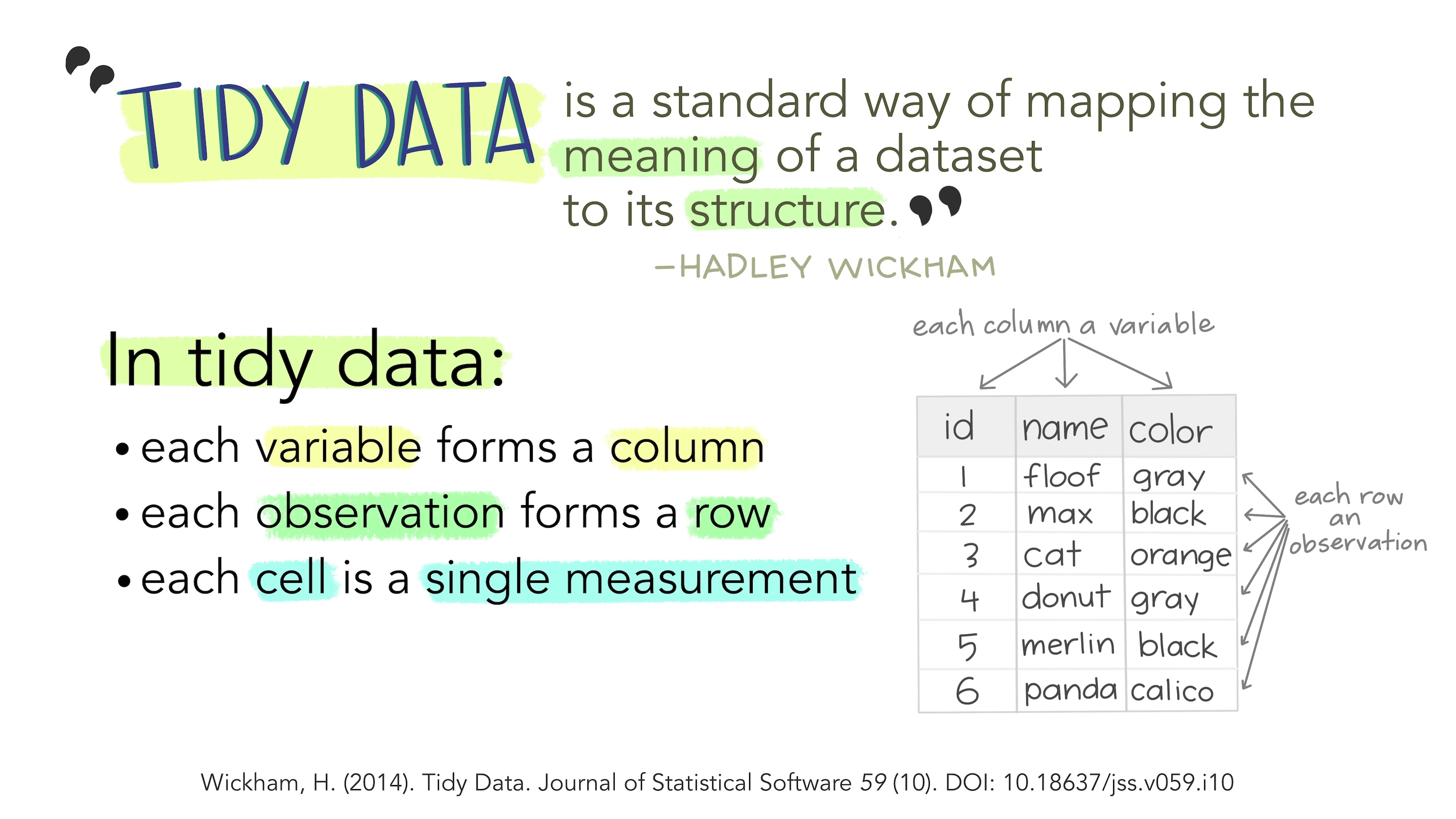
Wrangling is easier when data follows a consistent structure. Tidy data is a standard way of organizing a dataset so that every tool in the tidyverse — {dplyr}, {tidyr}, {ggplot2} — works on it the same way.

The three tidy rules:

1. Each variable forms a column
2. Each observation forms a row
3. Each cell contains a single measurement

Source: Tidy Data for reproducibility, efficiency, and collaboration

When data is tidy, the same tools work in the same ways across different datasets:

Source: Tidy Data for reproducibility, efficiency, and collaboration

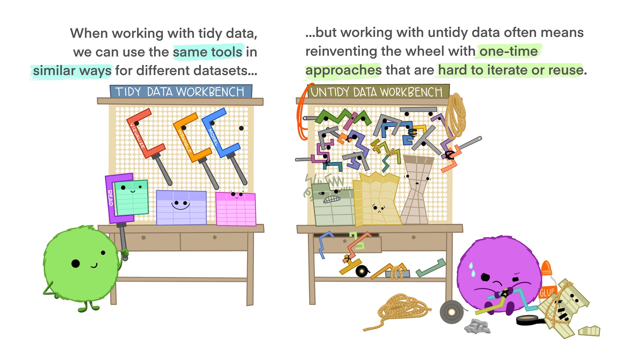
Untidy data comes in many forms — variables stored as column names, multiple variables crammed into one column, observations spread across multiple rows. {tidyr} provides tools to fix all of these.

Data reshaping with {tidyr}

NoteR for Data Science

This is a brief introduction to data tidying with {tidyr}. For a more comprehensive treatment, see R for Data Science.

Wide vs. long format

Data arrives in many shapes. Wide format has one row per subject with multiple measurement columns — it is often used in spreadsheets and reports. Long format has one row per subject-per-variable — it is what {ggplot2} and most statistical tools expect.

The relig_income dataset (built into {tidyr}) records survey respondents’ income levels by religious affiliation. Each row is a religion; each column beyond the first is an income bracket. This is wide format:

relig_income

# A tibble: 18 × 11
   religion           `<$10k` `$10-20k` `$20-30k` `$30-40k` `$40-50k` `$50-75k` `$75-100k`
   <chr>                <dbl>     <dbl>     <dbl>     <dbl>     <dbl>     <dbl>      <dbl>
 1 Agnostic                27        34        60        81        76       137        122
 2 Atheist                 12        27        37        52        35        70         73
 3 Buddhist                27        21        30        34        33        58         62
 4 Catholic               418       617       732       670       638      1116        949
 5 Don’t know/refused      15        14        15        11        10        35         21
 6 Evangelical Prot       575       869      1064       982       881      1486        949
 7 Hindu                    1         9         7         9        11        34         47
 8 Historically Blac…     228       244       236       238       197       223        131
 9 Jehovah's Witness       20        27        24        24        21        30         15
10 Jewish                  19        19        25        25        30        95         69
11 Mainline Prot          289       495       619       655       651      1107        939
12 Mormon                  29        40        48        51        56       112         85
13 Muslim                   6         7         9        10         9        23         16
14 Orthodox                13        17        23        32        32        47         38
15 Other Christian          9         7        11        13        13        14         18
16 Other Faiths            20        33        40        46        49        63         46
17 Other World Relig…       5         2         3         4         2         7          3
18 Unaffiliated           217       299       374       365       341       528        407
# ℹ 3 more variables: `$100-150k` <dbl>, `>150k` <dbl>, `Don't know/refused` <dbl>

The income information is spread across 10 columns. To plot this data with {ggplot2} — say, as a heat map with income on one axis and religion on the other — we need one column for income bracket and one for the count. We need to pivot to long format.

pivot_longer()

pivot_longer() gathers multiple columns into two: a names_to column (the column headers become values) and a values_to column (the cell values):

relig_long <- relig_income |>
  pivot_longer(
    cols = -religion,
    names_to = "income",
    values_to = "count"
  )
relig_long

1

cols = -religion means “pivot all columns except religion”. You can also specify columns by name, position, or with tidyselect helpers like starts_with().

2

names_to = "income" — the column names (<$10k, $10-20k, etc.) become values in a new column called income.

3

values_to = "count" — the cell values become values in a new column called count.

# A tibble: 180 × 3
   religion income             count
   <chr>    <chr>              <dbl>
 1 Agnostic <$10k                 27
 2 Agnostic $10-20k               34
 3 Agnostic $20-30k               60
 4 Agnostic $30-40k               81
 5 Agnostic $40-50k               76
 6 Agnostic $50-75k              137
 7 Agnostic $75-100k             122
 8 Agnostic $100-150k            109
 9 Agnostic >150k                 84
10 Agnostic Don't know/refused    96
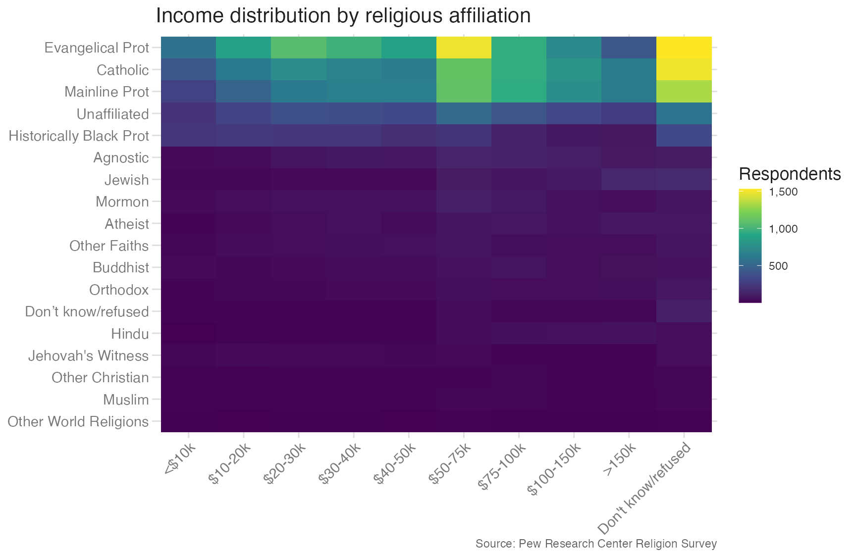
# ℹ 170 more rows

The result has one row per religion per income level. With data in long format, a tile chart is straightforward:

relig_long |>
  filter(religion != "Don't know/refused") |>
  mutate(
    income = fct_inorder(income),
    religion = fct_reorder(religion, count, sum)
  ) |>
  ggplot(aes(x = income, y = religion, fill = count)) +
  geom_tile() +
  scale_fill_viridis_c(labels = label_comma()) +
  scale_x_discrete(guide = guide_axis(angle = 45)) +
  labs(
    title = "Income distribution by religious affiliation",
    x = NULL,
    y = NULL,
    fill = "Respondents",
    caption = "Source: Pew Research Center Religion Survey"
  )

1

fct_inorder() preserves the original column order for income so the brackets read low-to-high left-to-right.

2

fct_reorder(religion, count, sum) sorts religions by total respondent count, putting the largest groups at the top.

When column names should become a numeric variable — as they would with year columns — use names_transform = parse_number inside pivot_longer():

df |>
  pivot_longer(
    cols = starts_with("year_"),
    names_to = "year",
    values_to = "value",
    names_transform = parse_number
  )

1

names_transform = parse_number converts the column names to numeric as part of the pivot, so the resulting column is <dbl> rather than <chr> and will be treated as a continuous variable on the x-axis.

pivot_wider()

The inverse operation is pivot_wider(). It converts long format back to wide, moving unique values from one column into separate columns:

relig_long |>
  pivot_wider(
    names_from = income,
    values_from = count
  )

1

names_from — take the unique values in this column and turn them into new column names.

2

values_from — fill in the new columns with values from this column.

# A tibble: 18 × 11
   religion           `<$10k` `$10-20k` `$20-30k` `$30-40k` `$40-50k` `$50-75k` `$75-100k`
   <chr>                <dbl>     <dbl>     <dbl>     <dbl>     <dbl>     <dbl>      <dbl>
 1 Agnostic                27        34        60        81        76       137        122
 2 Atheist                 12        27        37        52        35        70         73
 3 Buddhist                27        21        30        34        33        58         62
 4 Catholic               418       617       732       670       638      1116        949
 5 Don’t know/refused      15        14        15        11        10        35         21
 6 Evangelical Prot       575       869      1064       982       881      1486        949
 7 Hindu                    1         9         7         9        11        34         47
 8 Historically Blac…     228       244       236       238       197       223        131
 9 Jehovah's Witness       20        27        24        24        21        30         15
10 Jewish                  19        19        25        25        30        95         69
11 Mainline Prot          289       495       619       655       651      1107        939
12 Mormon                  29        40        48        51        56       112         85
13 Muslim                   6         7         9        10         9        23         16
14 Orthodox                13        17        23        32        32        47         38
15 Other Christian          9         7        11        13        13        14         18
16 Other Faiths            20        33        40        46        49        63         46
17 Other World Relig…       5         2         3         4         2         7          3
18 Unaffiliated           217       299       374       365       341       528        407
# ℹ 3 more variables: `$100-150k` <dbl>, `>150k` <dbl>, `Don't know/refused` <dbl>

The result is the original wide format. pivot_wider() is less commonly needed for visualization (most plots want long data) but is useful for creating summary tables and for reshaping data that arrives in a non-standard long format.

Summary

• {dplyr} provides verbs for transforming data: filter(), arrange(), select(), rename(), mutate(), group_by(), summarize(), and slice_*()
• Tidy data has one variable per column, one observation per row, and one value per cell — this structure is expected by {ggplot2} and most tidyverse tools
• pivot_longer() converts wide data to long format; pivot_wider() does the reverse
• Use names_transform = parse_number in pivot_longer() when column names represent a numeric variable (e.g., years)

Acknowledgements

Material derived in part from STA 313: Advanced Data Visualization and Data Science in a Box.