# packages for wrangling data and the original models
library(tidyverse)
library(tidymodels)
library(rcis)
library(patchwork)

# packages for model interpretation/explanation
library(DALEX)
library(DALEXtra)
library(lime)

# set random number generator seed value for reproducibility
set.seed(123)

theme_set(theme_minimal())Explain machine learning models: Predicting student debt
Suggested answers
Student debt in the United States has increased substantially over the past twenty years. In this application exercise we will interpret the results of a set of machine learning models predicting the median student debt load for students graduating in 2020-21 at four-year colleges and universities as a function of university-specific factors (e.g. public vs. private school, admissions rate, cost of attendance).
Load the documentation for rcis::scorecard to identify the variables used in the models.
Import models
We have estimated three distinct machine learning models to predict the median student debt load for students graduating in 2020-21 at four-year colleges and universities. Each model uses the same set of predictors, but the algorithms differ. Specifically, we have estimated
- Random forest
- Penalized regression
- 10-nearest neighbors
All models were estimated using tidymodels. We will load the training set, test set, and ML workflows from data/scorecard-models.Rdata.
# load Rdata file with all the data frames and pre-trained models
load("data/scorecard-models.RData")
Create explainer objects
In order to generate our interpretations, we will use the DALEX package. The first step in any DALEX operation is to create an explainer object. This object contains all the information needed to interpret the model’s predictions. We will create explainer objects for each of the three models.
Your turn: Review the syntax below for creating explainer objects using the explain_tidymodels() function. Then, create explainer objects for the random forest and \(k\) nearest neighbors models.
# use explain_*() to create explainer object
# first step of an DALEX operation
explainer_glmnet <- explain_tidymodels(
  model = glmnet_wf,
  # data should exclude the outcome feature
  data = scorecard_train |> select(-debt),
  # y should be a vector containing the outcome of interest for the training set
  y = scorecard_train$debt,
  # assign a label to clearly identify model in later plots
  label = "penalized regression"
)
Preparation of a new explainer is initiated
-> model label : penalized regression
-> data : 1288 rows 11 cols
-> data : tibble converted into a data.frame
-> target variable : 1288 values
-> predict function : yhat.workflow will be used ( default )
-> predicted values : No value for predict function target column. ( default )
-> model_info : package tidymodels , ver. 1.2.0 , task regression ( default )
-> predicted values : numerical, min = 5154.915 , mean = 16008.34 , max = 22749.84
-> residual function : difference between y and yhat ( default )
-> residuals : numerical, min = NA , mean = NA , max = NA
A new explainer has been created! # explainer for random forest model
explainer_rf <- explain_tidymodels(
model = rf_wf,
data = scorecard_train |> select(-debt),
y = scorecard_train$debt,
label = "random forest"
)Preparation of a new explainer is initiated
-> model label : random forest
-> data : 1288 rows 11 cols
-> data : tibble converted into a data.frame
-> target variable : 1288 values
-> predict function : yhat.workflow will be used ( default )
-> predicted values : No value for predict function target column. ( default )
-> model_info : package tidymodels , ver. 1.2.0 , task regression ( default )
-> predicted values : numerical, min = 5457.992 , mean = 15889.8 , max = 26682.32
-> residual function : difference between y and yhat ( default )
-> residuals : numerical, min = NA , mean = NA , max = NA
A new explainer has been created! # explainer for nearest neighbors model
explainer_kknn <- explain_tidymodels(
model = kknn_wf,
data = scorecard_train |> select(-debt),
y = scorecard_train$debt,
label = "k nearest neighbors"
)Preparation of a new explainer is initiated
-> model label : k nearest neighbors
-> data : 1288 rows 11 cols
-> data : tibble converted into a data.frame
-> target variable : 1288 values
-> predict function : yhat.workflow will be used ( default )
-> predicted values : No value for predict function target column. ( default )
-> model_info : package tidymodels , ver. 1.2.0 , task regression ( default )
-> predicted values : numerical, min = 5074.315 , mean = 16311.15 , max = 24000.65
-> residual function : difference between y and yhat ( default )
-> residuals : numerical, min = NA , mean = NA , max = NA
A new explainer has been created! Choose a couple of observations to explain
cornell <- filter(.data = scorecard, name == "Cornell University") |>
  select(-unitid, -name)
ic <- filter(.data = scorecard, name == "Ithaca College") |>
  select(-unitid, -name)
both <- bind_rows(cornell, ic)

# set row names for LIME later
rownames(both) <- c("Cornell University", "Ithaca College")
Shapley values
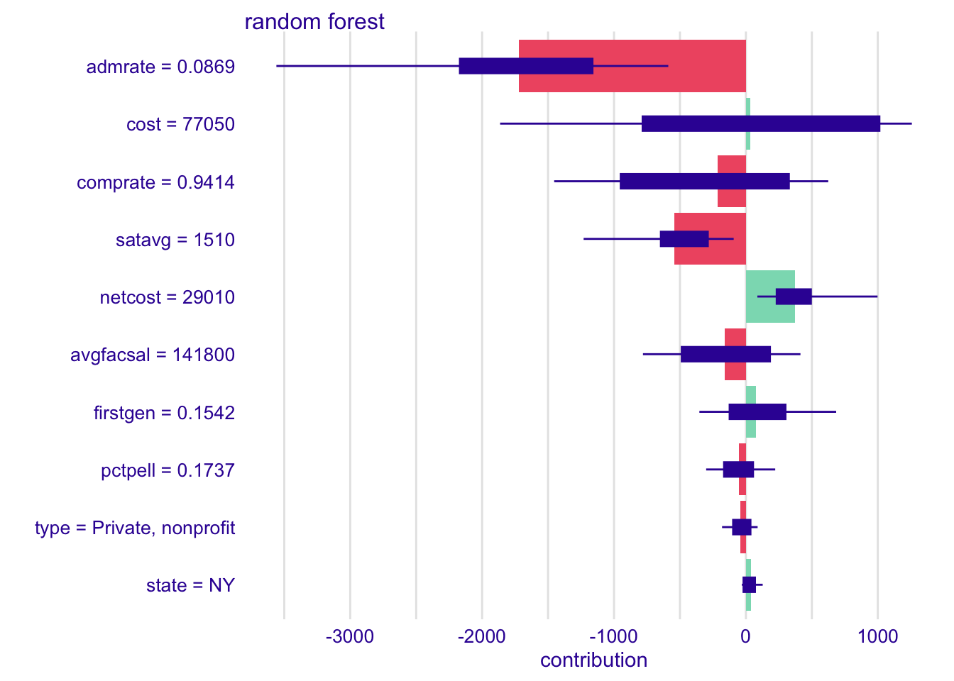
# explain Cornell with rf model
shap_cornell_rf <- predict_parts(
  explainer = explainer_rf,
  new_observation = cornell,
  type = "shap"
)
plot(shap_cornell_rf)
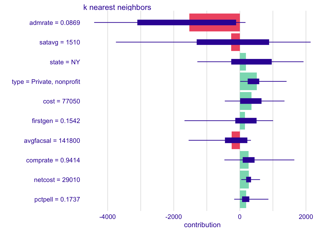
# explain Cornell with kknn model
shap_cornell_kknn <- predict_parts(
explainer = explainer_kknn,
new_observation = cornell,
type = "shap"
)
plot(shap_cornell_kknn)# increase the number of feature order permutations
shap_cornell_kknn_40 <- predict_parts(
explainer = explainer_kknn,
new_observation = cornell,
type = "shap",
B = 40
)
plot(shap_cornell_kknn_40)Pair with ggplot2
# based on example from https://www.tmwr.org/explain.html#local-explanations

shap_cornell_kknn |>
  # convert to pure tibble-formatted data frame
  as_tibble() |>
  # calculate average contribution per variable across permutations
  mutate(mean_val = mean(contribution), .by = variable) |>
  # reorder variable levels in order of absolute value of mean contribution
  mutate(variable = fct_reorder(variable, abs(mean_val))) |>
  # define basic ggplot object for horizontal boxplot
  ggplot(mapping = aes(x = contribution, y = variable, fill = mean_val > 0)) +
  # add a bar plot
  geom_col(
    data = ~ distinct(., variable, mean_val),
    mapping = aes(x = mean_val, y = variable),
    alpha = 0.5
  ) +
  # overlay with boxplot to show distribution
  geom_boxplot(width = 0.5) +
  # outcome variable is measured in dollars - contributions are the same units
  scale_x_continuous(labels = label_dollar()) +
  # use viridis color palette
  scale_fill_viridis_d(guide = "none") +
  labs(y = NULL)
Exercises
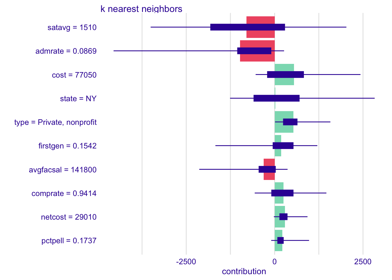
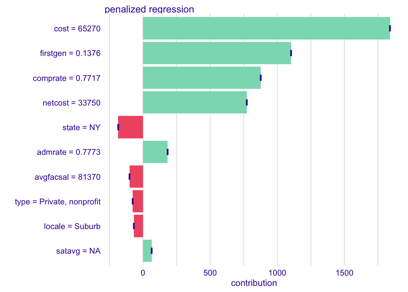
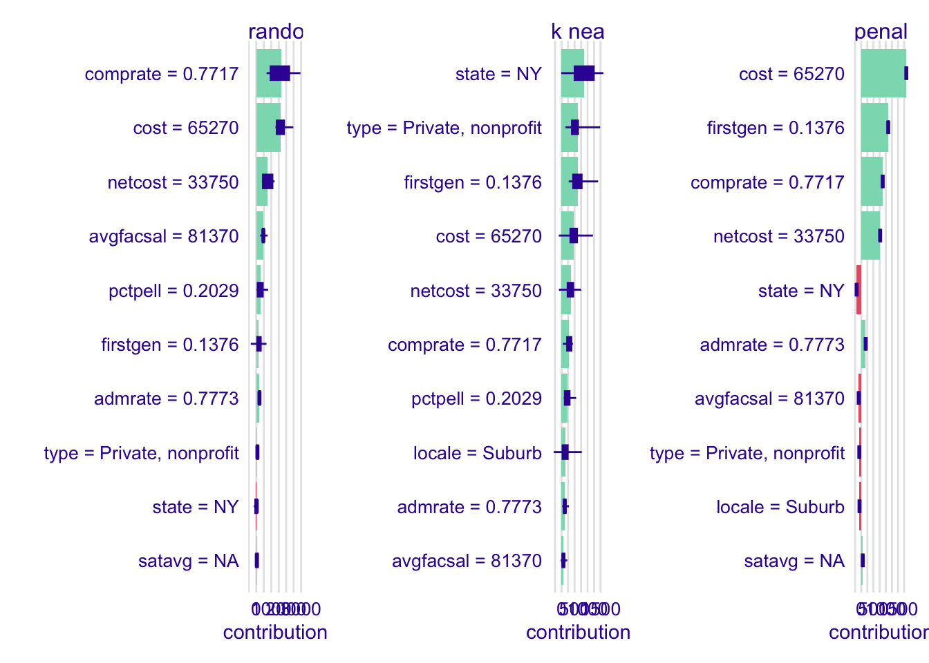
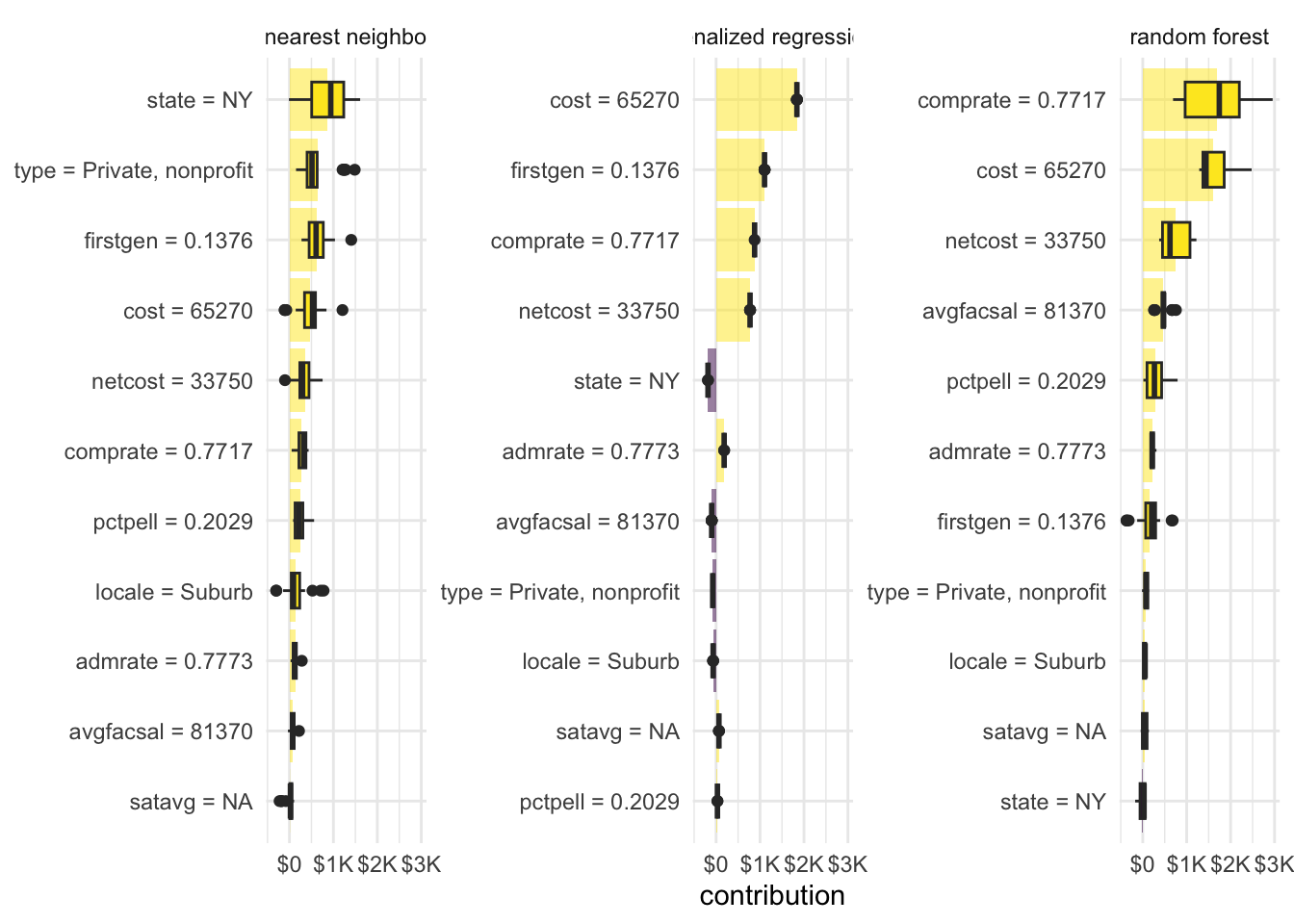
Your turn: Explain each model’s prediction for Ithaca College. How do they differ from each other?
# calculate shapley values
shap_ic_rf <- predict_parts(
  explainer = explainer_rf,
  new_observation = ic,
  type = "shap"
)

shap_ic_kknn <- predict_parts(
  explainer = explainer_kknn,
  new_observation = ic,
  type = "shap"
)

shap_ic_glmnet <- predict_parts(
  explainer = explainer_glmnet,
  new_observation = ic,
  type = "shap"
)
# generate plots for each
plot(shap_ic_rf)plot(shap_ic_kknn)plot(shap_ic_glmnet)# view side by side
plot(shap_ic_rf) +
plot(shap_ic_kknn) +
plot(shap_ic_glmnet)# or combine together and reuse ggplot code from above
bind_rows(
shap_ic_rf,
shap_ic_kknn,
shap_ic_glmnet
) |>
# convert to pure tibble-formatted data frame
as_tibble() |>
# calculate average contribution per variable across permutations
mutate(mean_val = mean(contribution), .by = c(label, variable)) |>
# reorder variable levels in order of absolute value of mean contribution
mutate(variable = tidytext::reorder_within(x = variable, by = abs(mean_val), within = label)) |>
# define basic ggplot object for horizontal boxplot
ggplot(mapping = aes(x = contribution, y = variable, fill = mean_val > 0)) +
# add a bar plot
geom_col(
data = ~ distinct(., label, variable, mean_val),
mapping = aes(x = mean_val, y = variable),
alpha = 0.5
) +
# overlay with boxplot to show distribution
geom_boxplot(width = 0.5) +
# facet for each model
facet_wrap(vars(label), scales = "free_y") +
tidytext::scale_y_reordered() +
# outcome variable is measured in dollars - contributions are the same units
scale_x_continuous(labels = label_dollar(scale_cut = cut_short_scale())) +
# use viridis color palette
scale_fill_viridis_d(guide = "none") +
labs(y = NULL)Add response here.
LIME
# prepare the recipe
prepped_rec_rf <- extract_recipe(rf_wf)

# write a function to bake the observation
bake_rf <- function(x) {
  bake(
    prepped_rec_rf,
    new_data = x
  )
}

# create explainer object
lime_explainer_rf <- lime(
  x = scorecard_train,
  model = extract_fit_parsnip(rf_wf),
  preprocess = bake_rf
)

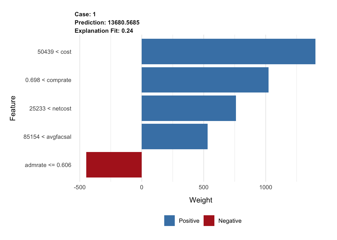
# top 5 features
explanation_rf <- explain(
  x = cornell,
  explainer = lime_explainer_rf,
  n_features = 5
)

plot_features(explanation_rf)
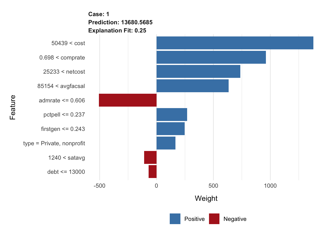
# top 10 features, increased permutations
explanation_rf <- explain(
x = cornell,
explainer = lime_explainer_rf,
n_features = 10,
n_permutations = 2000
)
plot_features(explanation_rf)A note on the penalized regression model
Due to how the model was trained, bake_glmnet() requires an additional composition argument. Otherwise everything else is the same.
# prepare the recipe
prepped_rec_glmnet <- extract_recipe(glmnet_wf)

# write a function to convert the legislative description to an appropriate matrix object
bake_glmnet <- function(x) {
  bake(
    prepped_rec_glmnet,
    new_data = x,
    composition = "dgCMatrix"
  )
}

# create explainer object
lime_explainer_glmnet <- lime(
  x = scorecard_train,
  model = extract_fit_parsnip(glmnet_wf),
  preprocess = bake_glmnet
)

# top 5 features
explanation_glmnet <- explain(
  x = cornell,
  explainer = lime_explainer_glmnet,
  n_features = 10
)

plot_features(explanation_glmnet)
Exercises
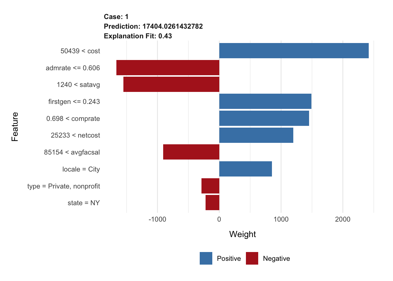
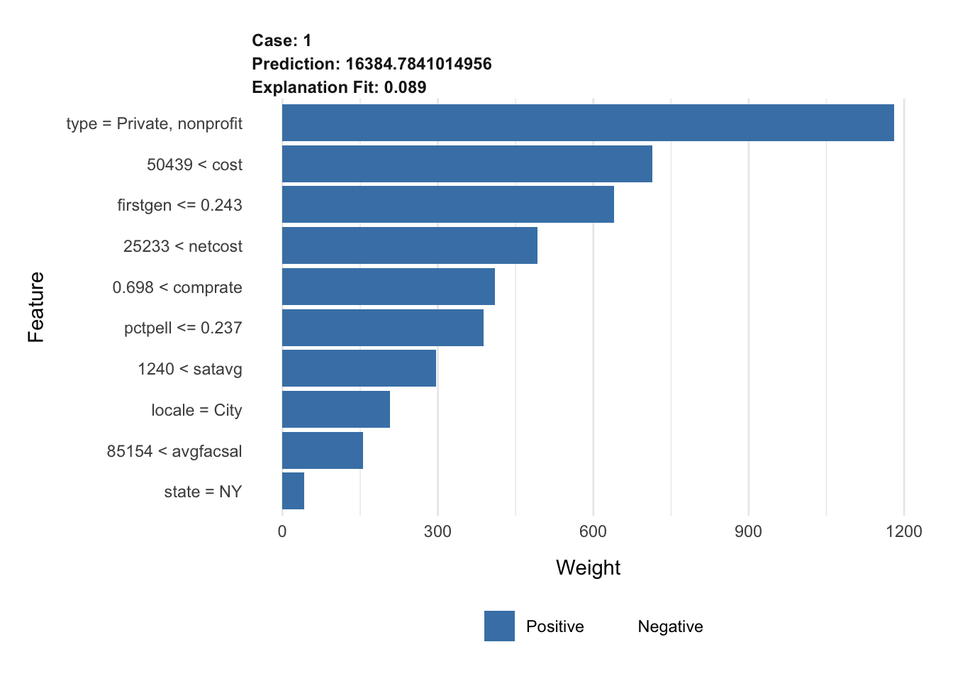
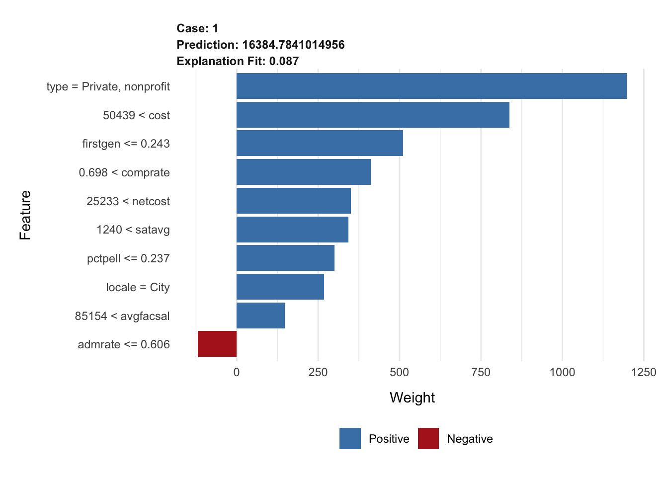
Your turn: Calculate a LIME explanation for Ithaca College and the \(k\) nearest neighbors model. What are the top 10 features? How well does the local model explain the prediction?
# prepare the recipe
prepped_rec_kknn <- extract_recipe(kknn_wf)

# write a function to bake the observation
bake_kknn <- function(x) {
  bake(
    prepped_rec_kknn,
    new_data = x
  )
}

# create explainer object
lime_explainer_kknn <- lime(
  x = scorecard_train,
  model = extract_fit_parsnip(kknn_wf),
  preprocess = bake_kknn
)

# top 10 features
explanation_kknn <- explain(
  x = cornell,
  explainer = lime_explainer_kknn,
  n_features = 10
)

plot_features(explanation_kknn)
Add response here.
Your turn: Reproduce the explanation but use a lasso model to select the most important features. How does the explanation change?
Choose your own adventure
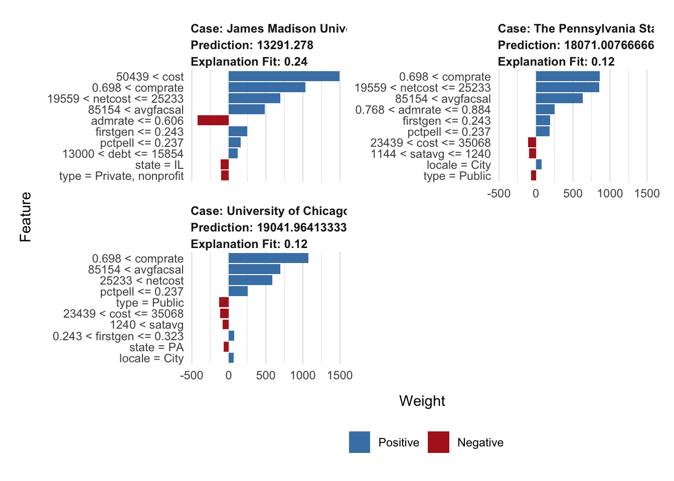
Your turn: Choose at least two other universities in the scorecard dataset. Generate explanations of their predicted median student debt from the random forest model using both SHAP and LIME. Compare the results. What are the most important features for each university? How do the explanations differ?
# choose institutions I have attended or worked at
my_obs <- filter(.data = scorecard, name %in% c(
  "James Madison University",
  "The Pennsylvania State University",
  "University of Chicago"
)) |>
  select(-unitid, -name)

# set row names for LIME later
rownames(my_obs) <- c(
  "James Madison University",
  "The Pennsylvania State University",
  "University of Chicago"
)
# calculate shapley values
shap_jmu <- predict_parts(
explainer = explainer_rf,
new_observation = my_obs[1, ],
type = "shap"
)
shap_penn_state <- predict_parts(
explainer = explainer_rf,
new_observation = my_obs[2, ],
type = "shap"
)
shap_uchi <- predict_parts(
explainer = explainer_rf,
new_observation = my_obs[3, ],
type = "shap"
)# or combine together and reuse ggplot code from above
bind_rows(
jmu = shap_jmu,
penn_state = shap_penn_state,
uchi = shap_uchi,
.id = "university"
) |>
# convert to pure tibble-formatted data frame
as_tibble() |>
# calculate average contribution per variable across permutations
group_by(university, variable) |>
mutate(mean_val = mean(contribution)) |>
ungroup() |>
# reorder variable levels in order of absolute value of mean contribution
mutate(variable = tidytext::reorder_within(x = variable, by = abs(mean_val), within = university)) |>
# define basic ggplot object for horizontal boxplot
ggplot(mapping = aes(x = contribution, y = variable, fill = mean_val > 0)) +
# add a bar plot
geom_col(
data = ~ distinct(., university, variable, mean_val),
mapping = aes(x = mean_val, y = variable),
alpha = 0.5
) +
# overlay with boxplot to show distribution
geom_boxplot(width = 0.5) +
# facet for each model
facet_wrap(vars(university), scales = "free_y") +
tidytext::scale_y_reordered() +
# outcome variable is measured in dollars - contributions are the same units
scale_x_continuous(labels = label_dollar(scale_cut = cut_short_scale())) +
# use viridis color palette
scale_fill_viridis_d(guide = "none") +
labs(y = NULL)# top 10 features, increased permutations
explanation_my_obs <- explain(
x = my_obs,
explainer = lime_explainer_rf,
n_features = 10,
n_permutations = 2000
)
plot_features(explanation_my_obs)Add response here.
sessioninfo::session_info()─ Session info ───────────────────────────────────────────────────────────────
setting value
version R version 4.3.2 (2023-10-31)
os macOS Ventura 13.6.6
system aarch64, darwin20
ui X11
language (EN)
collate en_US.UTF-8
ctype en_US.UTF-8
tz America/New_York
date 2024-04-29
pandoc 3.1.1 @ /Applications/RStudio.app/Contents/Resources/app/quarto/bin/tools/ (via rmarkdown)
─ Packages ───────────────────────────────────────────────────────────────────
package * version date (UTC) lib source
assertthat 0.2.1 2019-03-21 [1] CRAN (R 4.3.0)
backports 1.4.1 2021-12-13 [1] CRAN (R 4.3.0)
broom * 1.0.5 2023-06-09 [1] CRAN (R 4.3.0)
class 7.3-22 2023-05-03 [1] CRAN (R 4.3.2)
cli 3.6.2 2023-12-11 [1] CRAN (R 4.3.1)
codetools 0.2-19 2023-02-01 [1] CRAN (R 4.3.2)
colorspace 2.1-0 2023-01-23 [1] CRAN (R 4.3.0)
DALEX * 2.4.3 2023-01-15 [1] CRAN (R 4.3.0)
DALEXtra * 2.3.0 2023-05-26 [1] CRAN (R 4.3.0)
data.table 1.15.4 2024-03-30 [1] CRAN (R 4.3.1)
dials * 1.2.1 2024-02-22 [1] CRAN (R 4.3.1)
DiceDesign 1.10 2023-12-07 [1] CRAN (R 4.3.1)
digest 0.6.35 2024-03-11 [1] CRAN (R 4.3.1)
dplyr * 1.1.4 2023-11-17 [1] CRAN (R 4.3.1)
ellipsis 0.3.2 2021-04-29 [1] CRAN (R 4.3.0)
evaluate 0.23 2023-11-01 [1] CRAN (R 4.3.1)
fansi 1.0.6 2023-12-08 [1] CRAN (R 4.3.1)
farver 2.1.1 2022-07-06 [1] CRAN (R 4.3.0)
fastmap 1.1.1 2023-02-24 [1] CRAN (R 4.3.0)
forcats * 1.0.0 2023-01-29 [1] CRAN (R 4.3.0)
foreach 1.5.2 2022-02-02 [1] CRAN (R 4.3.0)
furrr 0.3.1 2022-08-15 [1] CRAN (R 4.3.0)
future 1.33.2 2024-03-26 [1] CRAN (R 4.3.1)
future.apply 1.11.2 2024-03-28 [1] CRAN (R 4.3.1)
generics 0.1.3 2022-07-05 [1] CRAN (R 4.3.0)
ggplot2 * 3.5.1 2024-04-23 [1] CRAN (R 4.3.1)
glmnet 4.1-8 2023-08-22 [1] CRAN (R 4.3.0)
globals 0.16.3 2024-03-08 [1] CRAN (R 4.3.1)
glue 1.7.0 2024-01-09 [1] CRAN (R 4.3.1)
gower 1.0.1 2022-12-22 [1] CRAN (R 4.3.0)
GPfit 1.0-8 2019-02-08 [1] CRAN (R 4.3.0)
gtable 0.3.5 2024-04-22 [1] CRAN (R 4.3.1)
hardhat 1.3.1 2024-02-02 [1] CRAN (R 4.3.1)
here 1.0.1 2020-12-13 [1] CRAN (R 4.3.0)
hms 1.1.3 2023-03-21 [1] CRAN (R 4.3.0)
htmltools 0.5.8.1 2024-04-04 [1] CRAN (R 4.3.1)
htmlwidgets 1.6.4 2023-12-06 [1] CRAN (R 4.3.1)
iBreakDown 2.1.2 2023-12-01 [1] CRAN (R 4.3.1)
igraph 1.6.0 2023-12-11 [1] CRAN (R 4.3.1)
infer * 1.0.7 2024-03-25 [1] CRAN (R 4.3.1)
ipred 0.9-14 2023-03-09 [1] CRAN (R 4.3.0)
iterators 1.0.14 2022-02-05 [1] CRAN (R 4.3.0)
janeaustenr 1.0.0 2022-08-26 [1] CRAN (R 4.3.0)
jsonlite 1.8.8 2023-12-04 [1] CRAN (R 4.3.1)
kknn 1.3.1 2016-03-26 [1] CRAN (R 4.3.0)
knitr 1.45 2023-10-30 [1] CRAN (R 4.3.1)
labeling 0.4.3 2023-08-29 [1] CRAN (R 4.3.0)
lattice 0.21-9 2023-10-01 [1] CRAN (R 4.3.2)
lava 1.8.0 2024-03-05 [1] CRAN (R 4.3.1)
lhs 1.1.6 2022-12-17 [1] CRAN (R 4.3.0)
lifecycle 1.0.4 2023-11-07 [1] CRAN (R 4.3.1)
lime * 0.5.3 2022-08-19 [1] CRAN (R 4.3.0)
listenv 0.9.1 2024-01-29 [1] CRAN (R 4.3.1)
lubridate * 1.9.3 2023-09-27 [1] CRAN (R 4.3.1)
magrittr 2.0.3 2022-03-30 [1] CRAN (R 4.3.0)
MASS 7.3-60 2023-05-04 [1] CRAN (R 4.3.2)
Matrix 1.6-1.1 2023-09-18 [1] CRAN (R 4.3.2)
modeldata * 1.3.0 2024-01-21 [1] CRAN (R 4.3.1)
munsell 0.5.1 2024-04-01 [1] CRAN (R 4.3.1)
nnet 7.3-19 2023-05-03 [1] CRAN (R 4.3.2)
parallelly 1.37.1 2024-02-29 [1] CRAN (R 4.3.1)
parsnip * 1.2.1 2024-03-22 [1] CRAN (R 4.3.1)
patchwork * 1.2.0 2024-01-08 [1] CRAN (R 4.3.1)
pillar 1.9.0 2023-03-22 [1] CRAN (R 4.3.0)
pkgconfig 2.0.3 2019-09-22 [1] CRAN (R 4.3.0)
prodlim 2023.08.28 2023-08-28 [1] CRAN (R 4.3.0)
purrr * 1.0.2 2023-08-10 [1] CRAN (R 4.3.0)
R6 2.5.1 2021-08-19 [1] CRAN (R 4.3.0)
ranger 0.16.0 2023-11-12 [1] CRAN (R 4.3.1)
rcis * 0.2.8 2024-01-09 [1] local
Rcpp 1.0.12 2024-01-09 [1] CRAN (R 4.3.1)
readr * 2.1.5 2024-01-10 [1] CRAN (R 4.3.1)
recipes * 1.0.10 2024-02-18 [1] CRAN (R 4.3.1)
rlang 1.1.3 2024-01-10 [1] CRAN (R 4.3.1)
rmarkdown 2.26 2024-03-05 [1] CRAN (R 4.3.1)
rpart 4.1.21 2023-10-09 [1] CRAN (R 4.3.2)
rprojroot 2.0.4 2023-11-05 [1] CRAN (R 4.3.1)
rsample * 1.2.1 2024-03-25 [1] CRAN (R 4.3.1)
rstudioapi 0.16.0 2024-03-24 [1] CRAN (R 4.3.1)
scales * 1.3.0 2023-11-28 [1] CRAN (R 4.3.1)
sessioninfo 1.2.2 2021-12-06 [1] CRAN (R 4.3.0)
shape 1.4.6.1 2024-02-23 [1] CRAN (R 4.3.1)
SnowballC 0.7.1 2023-04-25 [1] CRAN (R 4.3.0)
stringi 1.8.3 2023-12-11 [1] CRAN (R 4.3.1)
stringr * 1.5.1 2023-11-14 [1] CRAN (R 4.3.1)
survival 3.5-7 2023-08-14 [1] CRAN (R 4.3.2)
tibble * 3.2.1 2023-03-20 [1] CRAN (R 4.3.0)
tidymodels * 1.2.0 2024-03-25 [1] CRAN (R 4.3.1)
tidyr * 1.3.1 2024-01-24 [1] CRAN (R 4.3.1)
tidyselect 1.2.1 2024-03-11 [1] CRAN (R 4.3.1)
tidytext 0.4.1 2023-01-07 [1] CRAN (R 4.3.0)
tidyverse * 2.0.0 2023-02-22 [1] CRAN (R 4.3.0)
timechange 0.3.0 2024-01-18 [1] CRAN (R 4.3.1)
timeDate 4032.109 2023-12-14 [1] CRAN (R 4.3.1)
tokenizers 0.3.0 2022-12-22 [1] CRAN (R 4.3.0)
tune * 1.2.1 2024-04-18 [1] CRAN (R 4.3.1)
tzdb 0.4.0 2023-05-12 [1] CRAN (R 4.3.0)
utf8 1.2.4 2023-10-22 [1] CRAN (R 4.3.1)
vctrs 0.6.5 2023-12-01 [1] CRAN (R 4.3.1)
viridisLite 0.4.2 2023-05-02 [1] CRAN (R 4.3.0)
withr 3.0.0 2024-01-16 [1] CRAN (R 4.3.1)
workflows * 1.1.4 2024-02-19 [1] CRAN (R 4.3.1)
workflowsets * 1.1.0 2024-03-21 [1] CRAN (R 4.3.1)
xfun 0.43 2024-03-25 [1] CRAN (R 4.3.1)
yaml 2.3.8 2023-12-11 [1] CRAN (R 4.3.1)
yardstick * 1.3.1 2024-03-21 [1] CRAN (R 4.3.1)
[1] /Library/Frameworks/R.framework/Versions/4.3-arm64/Resources/library
──────────────────────────────────────────────────────────────────────────────
