# packages for wrangling data and the original models
library(tidyverse)
library(tidymodels)
library(rcis)

# packages for model interpretation/explanation
library(DALEX)
library(DALEXtra)
library(rattle) # fancy tree plots

# set random number generator seed value for reproducibility
set.seed(123)

theme_set(theme_minimal())Interpret machine learning models: Predicting student debt
Suggested answers
Application exercise
Answers
Student debt in the United States has increased substantially over the past twenty years. In this application exercise we will interpret the results of a set of machine learning models predicting the median student debt load for students graduating in 2020-21 at four-year colleges and universities as a function of university-specific factors (e.g. public vs. private school, admissions rate, cost of attendance).
Tip
Load the documentation for rcis::scorecard to identify the variables used in the models.
Import models
We have estimated three distinct machine learning models to predict the median student debt load for students graduating in 2020-21 at four-year colleges and universities. Each model uses the same set of predictors, but the algorithms differ. Specifically, we have estimated
- Random forest
- Penalized regression
- 10-nearest neighbors
All models were estimated using tidymodels. We will load the training set, test set, and ML workflows from data/scorecard-models.Rdata.
# load Rdata file with all the data frames and pre-trained models
load("data/scorecard-models.RData")
Create explainer objects
In order to generate our interpretations, we will use the DALEX package. The first step in any DALEX operation is to create an explainer object. This object contains all the information needed to interpret the model’s predictions. We will create explainer objects for each of the three models.
Your turn: Review the syntax below for creating explainer objects using the explain_tidymodels() function. Then, create explainer objects for the random forest and \(k\) nearest neighbors models.
# use explain_*() to create explainer object
# first step of an DALEX operation
explainer_glmnet <- explain_tidymodels(
  model = glmnet_wf,
  # data should exclude the outcome feature
  data = scorecard_train |> select(-debt),
  # y should be a vector containing the outcome of interest for the training set
  y = scorecard_train$debt,
  # assign a label to clearly identify model in later plots
  label = "penalized regression"
)
Preparation of a new explainer is initiated
-> model label : penalized regression
-> data : 1288 rows 11 cols
-> data : tibble converted into a data.frame
-> target variable : 1288 values
-> predict function : yhat.workflow will be used ( default )
-> predicted values : No value for predict function target column. ( default )
-> model_info : package tidymodels , ver. 1.2.0 , task regression ( default )
-> predicted values : numerical, min = 5154.915 , mean = 16008.34 , max = 22749.84
-> residual function : difference between y and yhat ( default )
-> residuals : numerical, min = NA , mean = NA , max = NA
A new explainer has been created! # explainer for random forest model
explainer_rf <- explain_tidymodels(
model = rf_wf,
data = scorecard_train |> select(-debt),
y = scorecard_train$debt,
label = "random forest"
)Preparation of a new explainer is initiated
-> model label : random forest
-> data : 1288 rows 11 cols
-> data : tibble converted into a data.frame
-> target variable : 1288 values
-> predict function : yhat.workflow will be used ( default )
-> predicted values : No value for predict function target column. ( default )
-> model_info : package tidymodels , ver. 1.2.0 , task regression ( default )
-> predicted values : numerical, min = 5457.992 , mean = 15889.8 , max = 26682.32
-> residual function : difference between y and yhat ( default )
-> residuals : numerical, min = NA , mean = NA , max = NA
A new explainer has been created! # explainer for nearest neighbors model
explainer_kknn <- explain_tidymodels(
model = kknn_wf,
data = scorecard_train |> select(-debt),
y = scorecard_train$debt,
label = "k nearest neighbors"
)Preparation of a new explainer is initiated
-> model label : k nearest neighbors
-> data : 1288 rows 11 cols
-> data : tibble converted into a data.frame
-> target variable : 1288 values
-> predict function : yhat.workflow will be used ( default )
-> predicted values : No value for predict function target column. ( default )
-> model_info : package tidymodels , ver. 1.2.0 , task regression ( default )
-> predicted values : numerical, min = 5074.315 , mean = 16311.15 , max = 24000.65
-> residual function : difference between y and yhat ( default )
-> residuals : numerical, min = NA , mean = NA , max = NA
A new explainer has been created! Permutation-based feature importance
The DALEX package provides a variety of methods for interpreting machine learning models. One common method is to calculate feature importance. Feature importance measures the contribution of each predictor variable to the model’s predictions. We will use the model_parts() function to calculate feature importance for the random forest model. It includes a built-in plot() method using ggplot2 to visualize the results.
# generate feature importance measures
vip_rf <- model_parts(explainer_rf)
vip_rf
variable mean_dropout_loss label
1 _full_model_ 1383.069 random forest
2 type 1548.168 random forest
3 locale 1551.794 random forest
4 satavg 1781.370 random forest
5 state 1793.858 random forest
6 admrate 1963.684 random forest
7 pctpell 2057.297 random forest
8 firstgen 2067.179 random forest
9 avgfacsal 2204.565 random forest
10 netcost 2439.938 random forest
11 comprate 2691.737 random forest
12 cost 2818.490 random forest
13 _baseline_ 5484.120 random forest# visualize feature importance
plot(vip_rf)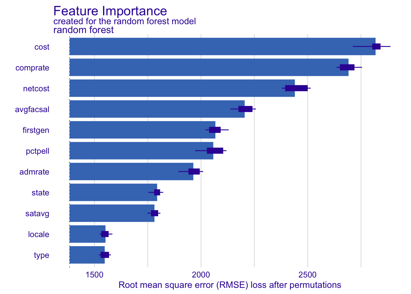
Your turn: Calculate feature importance for the random forest model using 100, 1000, and all observations for permutations. How does the compute time change?
# N = 100
system.time({
  model_parts(explainer_rf, N = 100)
})
user system elapsed
1.843 0.391 1.088 # default N = 1000
system.time({
model_parts(explainer_rf)
}) user system elapsed
9.410 0.901 2.362 # all observations
system.time({
model_parts(explainer_rf, N = NULL)
}) user system elapsed
11.302 1.066 2.617 Add response here. The larger the N, the longer it takes to compute feature importance.
Your turn: Calculate feature importance for the random forest model using the ratio of the raw change in the loss function. How does this differ from the raw change?
# calculate ratio rather than raw change
model_parts(explainer_rf, type = "ratio") |>
  plot()
Add response here. It expresses the impact of the feature in terms of a proportion or percentage change in the loss function rather than the original units.
Exercises
Your turn: Calculate feature importance for the penalized regression and \(k\) nearest neighbors using all observations for permutations. How do they compare to the random forest model?
# random forest model
vip_rf <- model_parts(explainer_rf, N = NULL)
plot(vip_rf)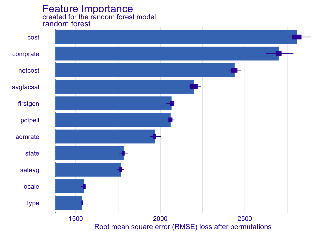
# compare to the glmnet model
vip_glmnet <- model_parts(explainer_glmnet, N = NULL)
plot(vip_glmnet)
# compare to the kknn model
vip_kknn <- model_parts(explainer_kknn, N = NULL)
plot(vip_kknn)
Add response here. Location of the university (state) matters much more in the penalized regression and nearest neighbor models. Frankly the feature importance seems to vary substantially across each of the models.
Your turn: Calculate feature importance for the random forest model three times using N = 100, changing the random seed value before each calculation. How do the results change? How does that compare to N = 1000?
# calculate random forest feature importance thrice
set.seed(123)
model_parts(explainer_rf, N = 100) |> plot()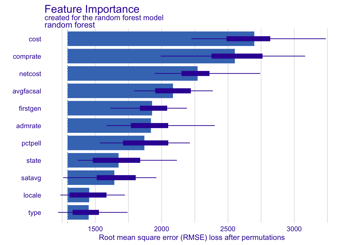
set.seed(234)
model_parts(explainer_rf, N = 100) |> plot()
set.seed(345)
model_parts(explainer_rf, N = 100) |> plot()
set.seed(123)
model_parts(explainer_rf, N = 1000) |> plot()
set.seed(234)
model_parts(explainer_rf, N = 1000) |> plot()
set.seed(345)
model_parts(explainer_rf, N = 1000) |> plot()
Add response here. Results vary somewhat when N = 100. Some of the features change order in the ranking. The distribution around the average is also much wider with a smaller N.
Partial dependence plots
In order to generate partial dependence plots, we will use model_profile(). This function calculates the average model prediction for a given variable while holding all other variables constant. We will generate partial dependence plots for the random forest model using the netcost variable.
# basic pdp for RF model and netcost variable
pdp_netcost <- model_profile(explainer_rf, variables = "netcost")
pdp_netcost
Top profiles :
_vname_ _label_ _x_ _yhat_ _ids_
1 netcost random forest 469.00 13996.66 0
2 netcost random forest 3213.62 13977.80 0
3 netcost random forest 4992.72 14240.02 0
4 netcost random forest 5538.12 14274.64 0
5 netcost random forest 6259.72 14354.71 0
6 netcost random forest 6723.70 14357.08 0We can visualize just the PDP, or the PDP with the ICE curves that underly the PDP.
# just the PDP
plot(pdp_netcost)
# PDP with ICE curves
plot(pdp_netcost, geom = "profiles")
By default model_profile() only uses 100 randomly selected observations to generate the profiles. Increasing the sample size may increase the quality of our estimate of the PDP, at the expense of a longer compute time.
# larger sample size
model_profile(explainer_rf, variables = "netcost", N = 500) |>
  plot(geom = "profiles")
We can also examine the PDP of a variable for distinct subgroups in the dataset. This is relevant for ML models which (either by design or the type of algorithm used) allow for interactions between predictor variables. In this case, we will examine the PDP of the net cost of attendance independently for public, private non-profit, and private for-profit institutions.
pdp_cost_group <- model_profile(explainer_rf, variables = "netcost", groups = "type")
plot(pdp_cost_group, geom = "profiles")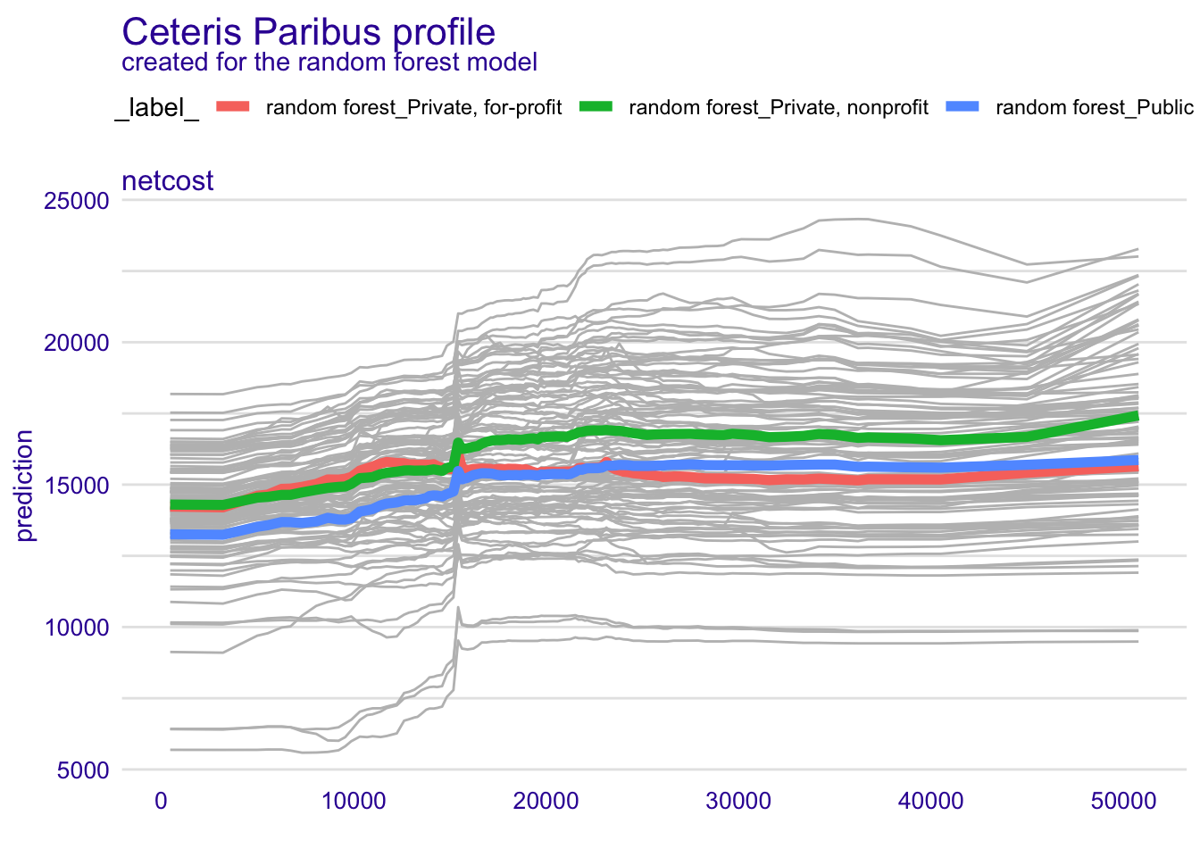
We also might want to generate a visualization directly from the aggregated profiles, rather than rely on DALEX to generate it for us.
# PDP for state - very hard to read
pdp_state_kknn <- model_profile(explainer_kknn, variables = "state")
plot(pdp_state_kknn)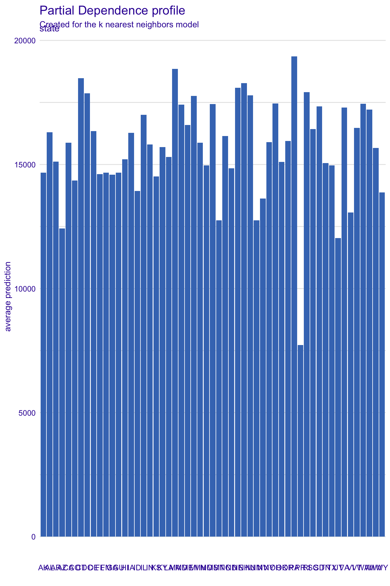
# examine the data structure
pdp_state_kknn
Top profiles :
_vname_ _label_ _x_ _yhat_ _ids_
1 state k nearest neighbors AK 14674.85 0
2 state k nearest neighbors AL 16296.66 0
3 state k nearest neighbors AR 15110.18 0
4 state k nearest neighbors AZ 12420.36 0
5 state k nearest neighbors CA 15881.41 0
6 state k nearest neighbors CO 14348.99 0# extract aggregated profiles
pdp_state_kknn$agr_profiles |>
# convert to tibble
as_tibble() |>
# reorder for plotting
mutate(`_x_` = fct_reorder(.f = `_x_`, .x = `_yhat_`)) |>
ggplot(mapping = aes(x = `_yhat_`, y = `_x_`, fill = `_yhat_`)) +
geom_col() +
scale_x_continuous(labels = label_dollar()) +
scale_fill_viridis_c(guide = "none") +
labs(
title = "Partial dependence plot for state",
subtitle = "Created for the k nearest neighbors model",
x = "Average prediction",
y = NULL
)
Exercises
Your turn: Create PDP + ICE curves for average faculty salary using all three models. How does the role of average faculty salary differ across the models?
# create PDP + ICE curves for avgfacsal from all three models
model_profile(explainer_rf, variables = "avgfacsal") |> plot(geom = "profiles")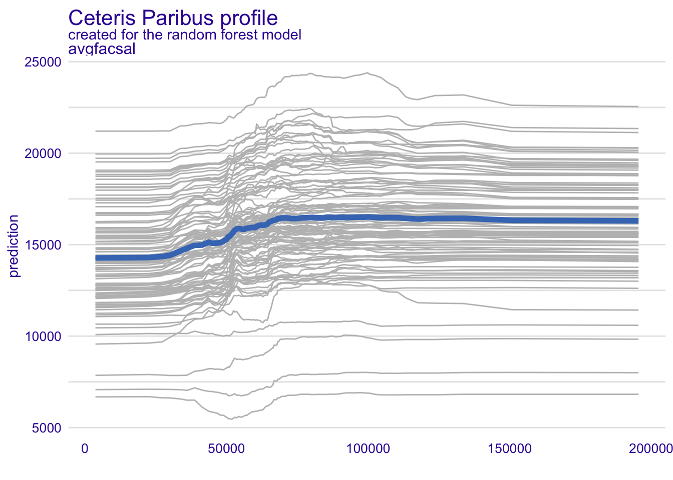
model_profile(explainer_glmnet, variables = "avgfacsal") |> plot(geom = "profiles")
model_profile(explainer_kknn, variables = "avgfacsal") |> plot(geom = "profiles")
Add response here. In the random forest model, the marginal effect of average faculty salary appears to be curvilinear. The predicted median debt load increases for average faculty salaries between $40K and $70K, then is relatively flat.
In the penalized regression model, the marginal effect of average faculty salary is linear and negative. In the nearest neighbors model the marginal effect is very flat, almost nothing.
Your turn: Create a PDP for all numeric variables in the penalized regression model. How do the variables compare in terms of their impact on the model?
# create PDP for all numeric variables in glmnet model
model_profile(explainer_glmnet, variables = NULL) |>
  plot()
Add response here. All the variables have a monotonic, linear relationship with the average model prediction. This is by definition since penalized regression still assumes a monotonic, linear relationship between the predictors and the outcome of interest.
Global surrogate models
In global surrogates, we estimate a simpler model to approximate the predictions of a more complex model. This can help us understand the relationships between the predictors and the outcome in the more complex model.
Demo: Fit a single decision tree to the predictions of the nearest neighbors model.
# get training set predictions from kknn model
kknn_train_preds <- bind_cols(
  scorecard_train,
  predict(kknn_wf, new_data = scorecard_train)
)

# fit a single decision tree to the training set predictions
gs_kknn_fit <- decision_tree(min_n = 40) |>
  set_mode("regression") |>
  fit(
    # exclude debt from the formula - it is the outcome of interest
    formula = .pred ~ . - debt,
    data = kknn_train_preds
  )

# evaluate the performance of the surrogate model
bind_cols(
  kknn_train_preds,
  predict(gs_kknn_fit, new_data = kknn_train_preds)
) |>
  # distinguish each prediction column - which model they came from
  rename(
    .pred_kknn = .pred...13,
    .pred_tree = .pred...14
  ) |>
  # estimate surrogate model performance
  metrics(truth = .pred_kknn, estimate = .pred_tree)
# A tibble: 3 × 3
.metric .estimator .estimate
<chr> <chr> <dbl>
1 rmse standard 1670.
2 rsq standard 0.697
3 mae standard 1309. fancyRpartPlot(gs_kknn_fit$fit,
sub = NULL,
palettes = "BuGn",
tweak = 2
)
Your turn: How well does the surrogate model explain the predictions of the nearest neighbors model? How do you interpret the predictions of the nearest neighbors model?
Add response here. Explains 70% of the variation in the nearest neighbors predictions. Overall, it seems that the location of the university (state), net cost of attendance, and completion rate are very important to making the predictions.
Session information
sessioninfo::session_info()─ Session info ───────────────────────────────────────────────────────────────
setting value
version R version 4.3.2 (2023-10-31)
os macOS Ventura 13.6.6
system aarch64, darwin20
ui X11
language (EN)
collate en_US.UTF-8
ctype en_US.UTF-8
tz America/New_York
date 2024-04-25
pandoc 3.1.1 @ /Applications/RStudio.app/Contents/Resources/app/quarto/bin/tools/ (via rmarkdown)
─ Packages ───────────────────────────────────────────────────────────────────
package * version date (UTC) lib source
backports 1.4.1 2021-12-13 [1] CRAN (R 4.3.0)
bitops * 1.0-7 2021-04-24 [1] CRAN (R 4.3.0)
broom * 1.0.5 2023-06-09 [1] CRAN (R 4.3.0)
class 7.3-22 2023-05-03 [1] CRAN (R 4.3.2)
cli 3.6.2 2023-12-11 [1] CRAN (R 4.3.1)
codetools 0.2-19 2023-02-01 [1] CRAN (R 4.3.2)
colorspace 2.1-0 2023-01-23 [1] CRAN (R 4.3.0)
DALEX * 2.4.3 2023-01-15 [1] CRAN (R 4.3.0)
DALEXtra * 2.3.0 2023-05-26 [1] CRAN (R 4.3.0)
data.table 1.15.4 2024-03-30 [1] CRAN (R 4.3.1)
dials * 1.2.1 2024-02-22 [1] CRAN (R 4.3.1)
DiceDesign 1.10 2023-12-07 [1] CRAN (R 4.3.1)
digest 0.6.35 2024-03-11 [1] CRAN (R 4.3.1)
dplyr * 1.1.4 2023-11-17 [1] CRAN (R 4.3.1)
ellipsis 0.3.2 2021-04-29 [1] CRAN (R 4.3.0)
evaluate 0.23 2023-11-01 [1] CRAN (R 4.3.1)
fansi 1.0.6 2023-12-08 [1] CRAN (R 4.3.1)
farver 2.1.1 2022-07-06 [1] CRAN (R 4.3.0)
fastmap 1.1.1 2023-02-24 [1] CRAN (R 4.3.0)
forcats * 1.0.0 2023-01-29 [1] CRAN (R 4.3.0)
foreach 1.5.2 2022-02-02 [1] CRAN (R 4.3.0)
furrr 0.3.1 2022-08-15 [1] CRAN (R 4.3.0)
future 1.33.2 2024-03-26 [1] CRAN (R 4.3.1)
future.apply 1.11.2 2024-03-28 [1] CRAN (R 4.3.1)
generics 0.1.3 2022-07-05 [1] CRAN (R 4.3.0)
ggplot2 * 3.5.1 2024-04-23 [1] CRAN (R 4.3.1)
glmnet 4.1-8 2023-08-22 [1] CRAN (R 4.3.0)
globals 0.16.3 2024-03-08 [1] CRAN (R 4.3.1)
glue 1.7.0 2024-01-09 [1] CRAN (R 4.3.1)
gower 1.0.1 2022-12-22 [1] CRAN (R 4.3.0)
GPfit 1.0-8 2019-02-08 [1] CRAN (R 4.3.0)
gtable 0.3.5 2024-04-22 [1] CRAN (R 4.3.1)
hardhat 1.3.1 2024-02-02 [1] CRAN (R 4.3.1)
here 1.0.1 2020-12-13 [1] CRAN (R 4.3.0)
hms 1.1.3 2023-03-21 [1] CRAN (R 4.3.0)
htmltools 0.5.8.1 2024-04-04 [1] CRAN (R 4.3.1)
htmlwidgets 1.6.4 2023-12-06 [1] CRAN (R 4.3.1)
igraph 1.6.0 2023-12-11 [1] CRAN (R 4.3.1)
infer * 1.0.7 2024-03-25 [1] CRAN (R 4.3.1)
ingredients 2.3.0 2023-01-15 [1] CRAN (R 4.3.0)
ipred 0.9-14 2023-03-09 [1] CRAN (R 4.3.0)
iterators 1.0.14 2022-02-05 [1] CRAN (R 4.3.0)
jsonlite 1.8.8 2023-12-04 [1] CRAN (R 4.3.1)
kknn 1.3.1 2016-03-26 [1] CRAN (R 4.3.0)
knitr 1.45 2023-10-30 [1] CRAN (R 4.3.1)
labeling 0.4.3 2023-08-29 [1] CRAN (R 4.3.0)
lattice 0.21-9 2023-10-01 [1] CRAN (R 4.3.2)
lava 1.8.0 2024-03-05 [1] CRAN (R 4.3.1)
lhs 1.1.6 2022-12-17 [1] CRAN (R 4.3.0)
lifecycle 1.0.4 2023-11-07 [1] CRAN (R 4.3.1)
listenv 0.9.1 2024-01-29 [1] CRAN (R 4.3.1)
lubridate * 1.9.3 2023-09-27 [1] CRAN (R 4.3.1)
magrittr 2.0.3 2022-03-30 [1] CRAN (R 4.3.0)
MASS 7.3-60 2023-05-04 [1] CRAN (R 4.3.2)
Matrix 1.6-1.1 2023-09-18 [1] CRAN (R 4.3.2)
modeldata * 1.3.0 2024-01-21 [1] CRAN (R 4.3.1)
munsell 0.5.1 2024-04-01 [1] CRAN (R 4.3.1)
nnet 7.3-19 2023-05-03 [1] CRAN (R 4.3.2)
parallelly 1.37.1 2024-02-29 [1] CRAN (R 4.3.1)
parsnip * 1.2.1 2024-03-22 [1] CRAN (R 4.3.1)
pillar 1.9.0 2023-03-22 [1] CRAN (R 4.3.0)
pkgconfig 2.0.3 2019-09-22 [1] CRAN (R 4.3.0)
prodlim 2023.08.28 2023-08-28 [1] CRAN (R 4.3.0)
purrr * 1.0.2 2023-08-10 [1] CRAN (R 4.3.0)
R6 2.5.1 2021-08-19 [1] CRAN (R 4.3.0)
ranger 0.16.0 2023-11-12 [1] CRAN (R 4.3.1)
rattle * 5.5.1 2022-03-21 [1] CRAN (R 4.3.0)
rcis * 0.2.8 2024-01-09 [1] local
RColorBrewer 1.1-3 2022-04-03 [1] CRAN (R 4.3.0)
Rcpp 1.0.12 2024-01-09 [1] CRAN (R 4.3.1)
readr * 2.1.5 2024-01-10 [1] CRAN (R 4.3.1)
recipes * 1.0.10 2024-02-18 [1] CRAN (R 4.3.1)
rlang 1.1.3 2024-01-10 [1] CRAN (R 4.3.1)
rmarkdown 2.26 2024-03-05 [1] CRAN (R 4.3.1)
rpart 4.1.21 2023-10-09 [1] CRAN (R 4.3.2)
rpart.plot 3.1.1 2022-05-21 [1] CRAN (R 4.3.0)
rprojroot 2.0.4 2023-11-05 [1] CRAN (R 4.3.1)
rsample * 1.2.1 2024-03-25 [1] CRAN (R 4.3.1)
rstudioapi 0.16.0 2024-03-24 [1] CRAN (R 4.3.1)
scales * 1.3.0 2023-11-28 [1] CRAN (R 4.3.1)
sessioninfo 1.2.2 2021-12-06 [1] CRAN (R 4.3.0)
shape 1.4.6.1 2024-02-23 [1] CRAN (R 4.3.1)
stringi 1.8.3 2023-12-11 [1] CRAN (R 4.3.1)
stringr * 1.5.1 2023-11-14 [1] CRAN (R 4.3.1)
survival 3.5-7 2023-08-14 [1] CRAN (R 4.3.2)
tibble * 3.2.1 2023-03-20 [1] CRAN (R 4.3.0)
tidymodels * 1.2.0 2024-03-25 [1] CRAN (R 4.3.1)
tidyr * 1.3.1 2024-01-24 [1] CRAN (R 4.3.1)
tidyselect 1.2.1 2024-03-11 [1] CRAN (R 4.3.1)
tidyverse * 2.0.0 2023-02-22 [1] CRAN (R 4.3.0)
timechange 0.3.0 2024-01-18 [1] CRAN (R 4.3.1)
timeDate 4032.109 2023-12-14 [1] CRAN (R 4.3.1)
tune * 1.2.1 2024-04-18 [1] CRAN (R 4.3.1)
tzdb 0.4.0 2023-05-12 [1] CRAN (R 4.3.0)
utf8 1.2.4 2023-10-22 [1] CRAN (R 4.3.1)
vctrs 0.6.5 2023-12-01 [1] CRAN (R 4.3.1)
viridisLite 0.4.2 2023-05-02 [1] CRAN (R 4.3.0)
withr 3.0.0 2024-01-16 [1] CRAN (R 4.3.1)
workflows * 1.1.4 2024-02-19 [1] CRAN (R 4.3.1)
workflowsets * 1.1.0 2024-03-21 [1] CRAN (R 4.3.1)
xfun 0.43 2024-03-25 [1] CRAN (R 4.3.1)
yaml 2.3.8 2023-12-11 [1] CRAN (R 4.3.1)
yardstick * 1.3.1 2024-03-21 [1] CRAN (R 4.3.1)
[1] /Library/Frameworks/R.framework/Versions/4.3-arm64/Resources/library
──────────────────────────────────────────────────────────────────────────────