AE 19: Increase in cost-burdened households in the United States
Suggested answers
We have already seen this semester that the cost of housing in the United States has been rising for several decades. A household is considered cost-burdened if they spend more than 30% of their income on housing costs.
In this application exercise we will explore trends in the percentage of cost-burdened rental households in the 10 largest core-based statistical areas (CBSAs).1 The relevant data can be found in data/cbsa-renters-burden.csv.
renter_burden <- read_csv(file = "data/cbsa-renters-burden.csv")
renter_burden
# A tibble: 190 × 4
year geoid name pct_burdened
<dbl> <dbl> <chr> <dbl>
1 2005 12060 Atlanta-Sandy Springs-Roswell, GA Metro Area 0.487
2 2005 16980 Chicago-Naperville-Elgin, IL-IN Metro Area 0.512
3 2005 19100 Dallas-Fort Worth-Arlington, TX Metro Area 0.480
4 2005 26420 Houston-Pasadena-The Woodlands, TX Metro Area 0.510
5 2005 31080 Los Angeles-Long Beach-Anaheim, CA Metro Area 0.556
6 2005 33100 Miami-Fort Lauderdale-West Palm Beach, FL Metro Area 0.608
7 2005 35620 New York-Newark-Jersey City, NY-NJ Metro Area 0.516
8 2005 37980 Philadelphia-Camden-Wilmington, PA-NJ-DE-MD Metro A… 0.511
9 2005 38060 Phoenix-Mesa-Chandler, AZ Metro Area 0.480
10 2005 47900 Washington-Arlington-Alexandria, DC-VA-MD-WV Metro … 0.467
# ℹ 180 more rowspct_burdened reports the percentage of renter-occupied housing units that spend 30%+ of their household income on gross rent.2
Communicating trends with a static visualization
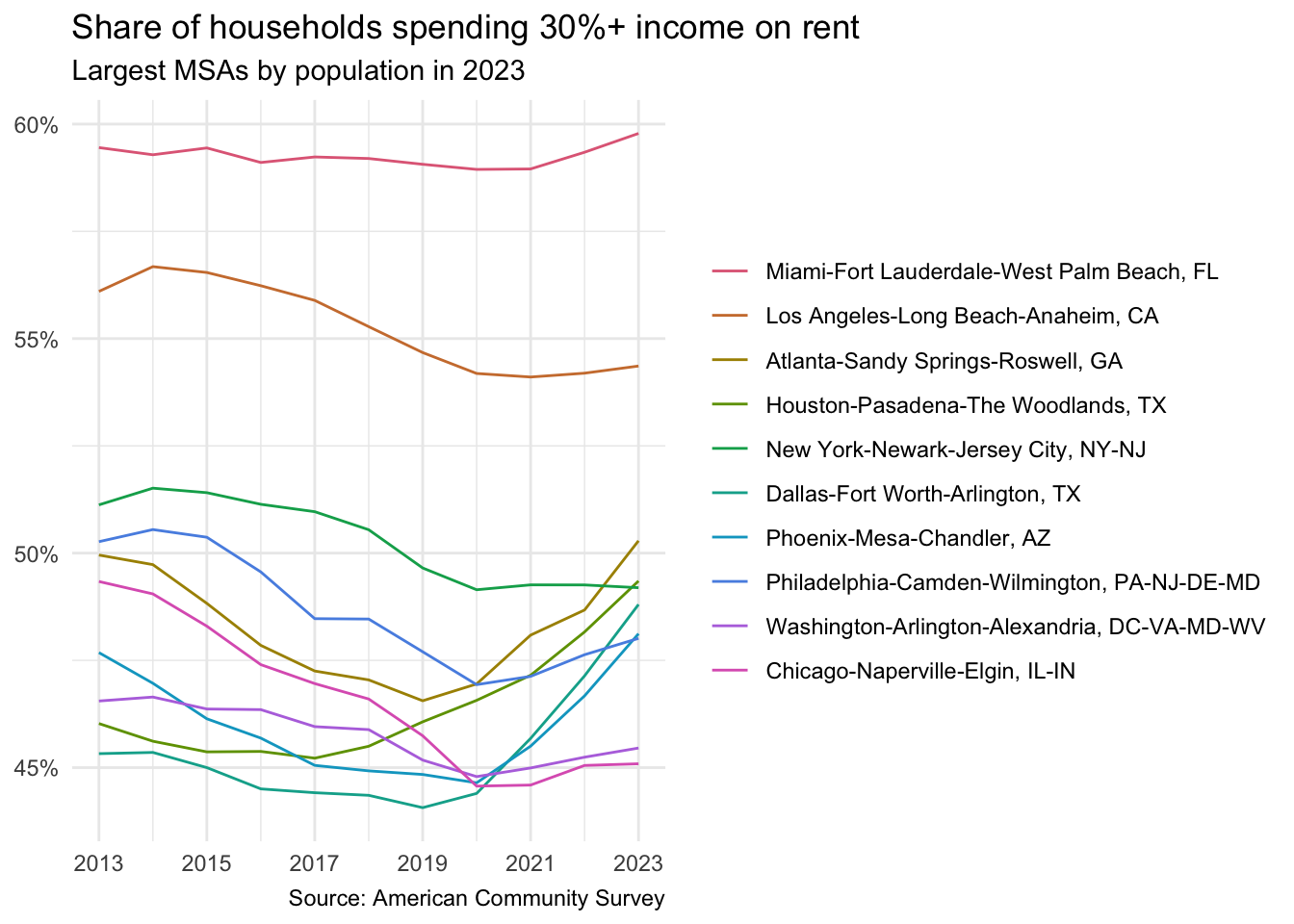
Your turn: While Americans face rising housing costs, the percentage of cost-burdened households has not increased uniformly across the country. Design and implement a static visualization to communicate the trends for these 10 CBSAs. Ensure it can reasonably be used to identify trends specific to each CBSA.
Using color to distinguish between CBSAs
# use color to distinguish between CBSAs
renter_burden |>
  # order the names by the most recent year for improved clarity in the legend
  mutate(name = fct_reorder2(.f = name, .x = year, .y = pct_burdened)) |>
  ggplot(mapping = aes(x = year, y = pct_burdened, color = name)) +
  geom_line() +
  scale_y_continuous(labels = label_percent()) +
  scale_color_discrete_qualitative() +
  labs(
    x = NULL,
    y = NULL,
    color = NULL,
    title = "Share of households spending 30%+ income on rent",
    subtitle = "Largest metro regions by population in 2024",
    caption = "Source: American Community Survey"
  )
Add direct labels
# set seed for reproducibility
set.seed(123)
ggplot(
  data = renter_burden,
  mapping = aes(x = year, y = pct_burdened, group = name)
) +
  geom_line() +
  # just label the last year in the data
  geom_text_repel(
    data = renter_burden |>
      slice_max(order_by = year, n = 1, by = geoid),
    # wrap the character strings for space
    mapping = aes(label = str_wrap(name, width = 30)),
    # move labels over 25 units to the right before repelling them
    nudge_x = 25,
    # left alignment of text
    hjust = 0,
    segment.color = "grey70"
  ) +
  # adjust x-axis breaks
  scale_x_continuous(breaks = seq(from = 2005, to = 2025, by = 5)) +
  scale_y_continuous(labels = label_percent()) +
  labs(
    x = NULL,
    y = NULL,
    title = "Share of households spending 30%+ income on rent",
    subtitle = "Largest metro regions by population in 2024",
    caption = "Source: American Community Survey"
  ) +
  theme(panel.grid.minor = element_blank())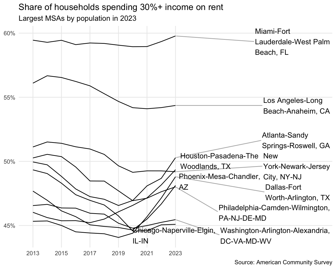
Communicating trends with an interactive visualization
Your turn: Design and implement an interactive visualization to communicate the trends for these 10 CBSAs. Ensure it can reasonably be used to identify trends specific to each CBSA. Leverage interactive components to reduce clutter in the visualization and effectively utilize interactivity.
- Using
geom_line_interactive()andgeom_point_interactive() - Customizing the tooltip to provide better-formatted information
- Using
girafe_options()to emphasize the hovered CBSA
Using {ggiraph} and customizing the tooltip
interactive_burden <- renter_burden |>
  mutate(
    name = fct_reorder2(.f = name, .x = year, .y = pct_burdened),
    # create a more informative tooltip
    tooltip = str_glue(
      "<span style='font-weight:bold;'>{name}</span><br>Year: {year}<br>Share of cost-burdened renters: {label_percent(accuracy = 0.1)(pct_burdened)}"
    )
  )

p <- interactive_burden |>
  ggplot(
    mapping = aes(x = year, y = pct_burdened, group = name, color = name)
  ) +
  # interactive line layer
  geom_line_interactive(
    mapping = aes(
      data_id = name,
      # format tooltips using bold font, same as the points
      tooltip = str_glue("<span style='font-weight:bold;'>{name}</span>")
    ),
    # increase linewidth and make lines more transparent to improve hover effect
    linewidth = 0.9,
    alpha = 0.8
  ) +
  # interactive point layer
  geom_point_interactive(
    mapping = aes(data_id = name, tooltip = tooltip),
    # increase points to enlarge hover area
    size = 2.2
  ) +
  scale_y_continuous(labels = label_percent()) +
  scale_color_discrete_qualitative(guide = "none") +
  labs(
    x = NULL,
    y = NULL,
    title = "Share of households spending 30%+ income on rent",
    subtitle = "Largest metro regions by population in 2024",
    caption = "Source: American Community Survey"
  )

girafe(ggobj = p) |>
  girafe_options(
    # make the hovered line thicker
    opts_hover(css = "stroke-width: 3.5px;"),
    # increase the transparency of non-hovered lines
    opts_hover_inv(css = "opacity: 0.15;"),
    # format the tooltips
    opts_tooltip(
      css = str_c(
        "background-color: white;",
        "color: #222000;",
        "padding: 0.4rem 0.6rem;",
        "border: 1px solid #d9d9d9;",
        "border-radius: 0.25rem;"
      )
    )
)sessioninfo::session_info()─ Session info ───────────────────────────────────────────────────────────────
setting value
version R version 4.5.2 (2025-10-31)
os macOS Tahoe 26.4.1
system aarch64, darwin20
ui X11
language (EN)
collate en_US.UTF-8
ctype en_US.UTF-8
tz America/New_York
date 2026-04-10
pandoc 3.4 @ /usr/local/bin/ (via rmarkdown)
quarto 1.9.36 @ /usr/local/bin/quarto
─ Packages ───────────────────────────────────────────────────────────────────
! package * version date (UTC) lib source
P bit 4.6.0 2025-03-06 [?] RSPM (R 4.5.0)
P bit64 4.6.0-1 2025-01-16 [?] RSPM (R 4.5.0)
P cli 3.6.5 2025-04-23 [?] RSPM (R 4.5.0)
P colorspace * 2.1-2 2025-09-22 [?] RSPM
P crayon 1.5.3 2024-06-20 [?] RSPM (R 4.5.0)
P digest 0.6.39 2025-11-19 [?] RSPM (R 4.5.0)
P dplyr * 1.2.0 2026-02-03 [?] RSPM
P evaluate 1.0.5 2025-08-27 [?] RSPM (R 4.5.0)
P farver 2.1.2 2024-05-13 [?] RSPM (R 4.5.0)
P fastmap 1.2.0 2024-05-15 [?] RSPM (R 4.5.0)
P fontBitstreamVera 0.1.1 2017-02-01 [?] RSPM
P fontLiberation 0.1.0 2016-10-15 [?] RSPM
P fontquiver 0.2.1 2017-02-01 [?] RSPM
P forcats * 1.0.1 2025-09-25 [?] RSPM (R 4.5.0)
P gdtools 0.5.0 2026-02-09 [?] RSPM
P generics 0.1.4 2025-05-09 [?] RSPM (R 4.5.0)
P ggiraph * 0.9.6 2026-02-21 [?] url (https://cran.r-project.org/bin/macosx/big-sur-arm64/contrib/4.5/ggiraph_0.9.6.tgz)
P ggplot2 * 4.0.1 2025-11-14 [?] RSPM (R 4.5.0)
P ggrepel * 0.9.6 2024-09-07 [?] RSPM (R 4.5.0)
P glue 1.8.0 2024-09-30 [?] RSPM (R 4.5.0)
P gtable 0.3.6 2024-10-25 [?] RSPM (R 4.5.0)
P here 1.0.2 2025-09-15 [?] CRAN (R 4.5.0)
P hms 1.1.4 2025-10-17 [?] RSPM (R 4.5.0)
P htmltools 0.5.9 2025-12-04 [?] RSPM (R 4.5.0)
P htmlwidgets 1.6.4 2023-12-06 [?] RSPM (R 4.5.0)
P jsonlite 2.0.0 2025-03-27 [?] RSPM (R 4.5.0)
P knitr 1.51 2025-12-20 [?] RSPM (R 4.5.0)
P labeling 0.4.3 2023-08-29 [?] RSPM (R 4.5.0)
P lifecycle 1.0.5 2026-01-08 [?] RSPM (R 4.5.0)
P lubridate * 1.9.4 2024-12-08 [?] RSPM (R 4.5.0)
P magrittr 2.0.4 2025-09-12 [?] RSPM (R 4.5.0)
P MASS 7.3-65 2025-02-28 [?] CRAN (R 4.5.2)
P otel 0.2.0 2025-08-29 [?] RSPM (R 4.5.0)
P pillar 1.11.1 2025-09-17 [?] RSPM (R 4.5.0)
P pkgconfig 2.0.3 2019-09-22 [?] RSPM (R 4.5.0)
P purrr * 1.2.0 2025-11-04 [?] CRAN (R 4.5.0)
P R6 2.6.1 2025-02-15 [?] RSPM (R 4.5.0)
P RColorBrewer 1.1-3 2022-04-03 [?] RSPM (R 4.5.0)
P Rcpp 1.1.0 2025-07-02 [?] RSPM (R 4.5.0)
P readr * 2.1.6 2025-11-14 [?] RSPM (R 4.5.0)
P renv 1.2.0 2026-03-25 [?] RSPM
P rlang 1.1.7 2026-01-09 [?] RSPM (R 4.5.0)
P rmarkdown 2.30 2025-09-28 [?] RSPM (R 4.5.0)
P rprojroot 2.1.1 2025-08-26 [?] RSPM (R 4.5.0)
P S7 0.2.1 2025-11-14 [?] RSPM (R 4.5.0)
P scales * 1.4.0 2025-04-24 [?] RSPM (R 4.5.0)
P sessioninfo 1.2.3 2025-02-05 [?] RSPM (R 4.5.0)
P stringi 1.8.7 2025-03-27 [?] RSPM (R 4.5.0)
P stringr * 1.6.0 2025-11-04 [?] RSPM (R 4.5.0)
P systemfonts 1.3.1 2025-10-01 [?] RSPM (R 4.5.0)
P tibble * 3.3.0 2025-06-08 [?] RSPM (R 4.5.0)
P tidyr * 1.3.2 2025-12-19 [?] RSPM (R 4.5.0)
P tidyselect 1.2.1 2024-03-11 [?] RSPM (R 4.5.0)
P tidyverse * 2.0.0 2023-02-22 [?] RSPM (R 4.5.0)
P timechange 0.3.0 2024-01-18 [?] RSPM (R 4.5.0)
P tzdb 0.5.0 2025-03-15 [?] RSPM (R 4.5.0)
P utf8 1.2.6 2025-06-08 [?] RSPM (R 4.5.0)
P vctrs 0.7.1 2026-01-23 [?] RSPM
P vroom 1.6.7 2025-11-28 [?] RSPM (R 4.5.0)
P withr 3.0.2 2024-10-28 [?] RSPM (R 4.5.0)
P xfun 0.55 2025-12-16 [?] CRAN (R 4.5.2)
P yaml 2.3.12 2025-12-10 [?] RSPM (R 4.5.0)
[1] /Users/bcs88/Projects/info-3312/course-site/renv/library/macos/R-4.5/aarch64-apple-darwin20
[2] /Users/bcs88/Library/Caches/org.R-project.R/R/renv/sandbox/macos/R-4.5/aarch64-apple-darwin20/4cd76b74
* ── Packages attached to the search path.
P ── Loaded and on-disk path mismatch.
──────────────────────────────────────────────────────────────────────────────Footnotes
Based on population as of 2024.↩︎
Specifically Table B25070 from the American Community Survey.↩︎