library(tidyverse)
library(tidymodels)
library(marginaleffects)
library(scales)
library(colorspace)

theme_set(theme_minimal())Interpreting regression models through marginal effects
Suggested answers
Application exercise
Answers
Studying public corruption
Political scientists are frequently concerned with issues related to corruption and human rights. In this application exercise, we’ll use data from the World Bank and the Varieties of Democracy project to study the relationship between respect for human rights, public sector corruption, and legal campaign finance disclosure requirements.
Import data
# import corruption data
corruption <- read_rds(file = "data/corruption.rds")
glimpse(corruption)
Rows: 169
Columns: 17
$ country_name <chr> "Mexico", "Suriname", "Sweden", "Switzerland"…
$ country_text_id <chr> "MEX", "SUR", "SWE", "CHE", "GHA", "ZAF", "JP…
$ year <dbl> 2020, 2020, 2020, 2020, 2020, 2020, 2020, 202…
$ region <fct> Latin America and the Caribbean, Latin Americ…
$ disclose_donations_ord <dbl> 3, 1, 3, 0, 2, 2, 3, 2, 2, 2, 2, 0, 3, 3, 4, …
$ public_sector_corruption <dbl> 49.1, 24.4, 1.5, 1.2, 66.6, 58.0, 3.8, 37.7, …
$ polyarchy <dbl> 65.2, 75.4, 90.1, 90.1, 72.2, 71.4, 83.5, 42.…
$ civil_liberties <dbl> 70.2, 86.7, 96.5, 95.3, 91.7, 83.0, 91.3, 49.…
$ disclose_donations <lgl> TRUE, FALSE, TRUE, FALSE, FALSE, FALSE, TRUE,…
$ iso2c <chr> "MX", "SR", "SE", "CH", "GH", "ZA", "JP", "MM…
$ population <dbl> 125998302, 607065, 10353442, 8638167, 3218040…
$ gdp_percapita <dbl> 9273.811, 7275.365, 51952.673, 84637.013, 195…
$ capital <chr> "Mexico City", "Paramaribo", "Stockholm", "Be…
$ longitude <chr> "-99.1276", "-55.1679", "18.0645", "7.44821",…
$ latitude <chr> "19.427", "5.8232", "59.3327", "46.948", "5.5…
$ income <chr> "Upper middle income", "Upper middle income",…
$ log_gdp_percapita <dbl> 9.134950, 8.892249, 10.858088, 11.346127, 7.5…The dataset covers 169 countries in 2020. The main variables we will utilize include:
public_sector_corruption- Index of public sector corruption, ranging from 0 to 100, based on the measureTo what extent do public sector employees grant favors in exchange for bribes, kickbacks, or other material inducements, and how often do they steal, embezzle, or misappropriate public funds or other state resources for personal or family use?
0 indicates no corruption and 100 the most corruption.
disclosure_donations- Presence of campaign finance disclosure laws, coded asFALSEfor no (none or minimally enforced disclosure requirements) andTRUEfor yes (disclosure requirements in place and largely enforced).polyarchy- continuous variable from 0 to 100 with higher values representing greater achievement of democratic ideals.civil_liberties- Index of civil liberties, ranging from 0 to 100, with higher values representing better respect for human rights and civil liberties.log_gdp_percapita- natural logarithm of GDP per capita in constant 2015 USD.region- region of the world where the country is located. One of- Eastern Europe and Central Asia (including Mongolia)
- Latin America and the Caribbean
- The Middle East and North Africa (including Israel and Turkey, excluding Cyprus)
- Sub-Saharan Africa
- Western Europe and North America (including Cyprus, Australia and New Zealand)
- Asia and Pacific (excluding Australia and New Zealand)
Effect of civil liberties on public sector corruption
First let’s examine the effect of civil liberties on public sector corruption.
Demo: Estimate a simple linear regression model of the effect of civil liberties on public sector corruption.
# simple model
ggplot(data = corruption, mapping = aes(x = civil_liberties, y = public_sector_corruption)) +
  geom_point() +
  geom_smooth(method = "lm") +
  labs(
    x = "Civil liberties index",
    y = "Public sector corruption index"
  )
# estimate formally
model_simple <- linear_reg() |>
  fit(public_sector_corruption ~ civil_liberties,
    data = corruption
  ) |>
  extract_fit_engine()
tidy(model_simple)
# A tibble: 2 × 5
term estimate std.error statistic p.value
<chr> <dbl> <dbl> <dbl> <dbl>
1 (Intercept) 102. 5.36 19.1 7.90e-44
2 civil_liberties -0.813 0.0734 -11.1 1.04e-21Your turn: Interpret the results. What do we learn from this model in terms of the strength and directionality of the relationship?
Add response here. Higher civil liberties scores are associated with lower public sector corruption scores. Looks like a relatively strong relationship. Seems to be statistically significant based on the 95% CI printed by ggplot2.
Add a polynomial term
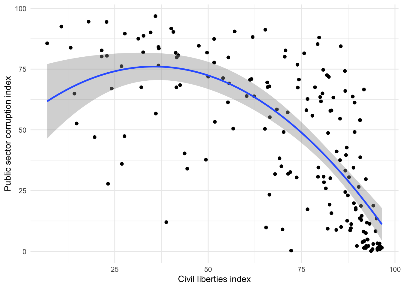
Demo: Estimate a polynomial linear regression model of the effect of civil liberties on public sector corruption.
# visualize the model
ggplot(data = corruption, mapping = aes(x = civil_liberties, y = public_sector_corruption)) +
  geom_point() +
  geom_smooth(method = "lm", formula = y ~ x + I(x^2)) +
  labs(
    x = "Civil liberties index",
    y = "Public sector corruption index"
  )
# estimate the model
model_sq <- linear_reg() |>
  fit(public_sector_corruption ~ civil_liberties + I(civil_liberties^2),
    data = corruption
  ) |>
  extract_fit_engine()
tidy(model_sq)
# A tibble: 3 × 5
term estimate std.error statistic p.value
<chr> <dbl> <dbl> <dbl> <dbl>
1 (Intercept) 54.0 10.1 5.37 0.000000263
2 civil_liberties 1.24 0.378 3.29 0.00124
3 I(civil_liberties^2) -0.0175 0.00316 -5.53 0.000000125Your turn: Interpret the results. What do we learn from this model in terms of the strength and directionality of the relationship?
Add response here. The relationship between civil liberties and public sector corruption is not linear. For lower civil liberties scores public sector corruption is expected to be high and with (maybe) a slight positive relationship. For higher civil liberties scores above approximately 30, there is a strong negative relationship with public sector corruption.
What is the marginal effect of civil liberties on public sector corruption?
Demo: What is the marginal effect of civil liberties on public sector corruption for countries with civil liberties scores of 25, 55, and 80?
slopes(
  model_sq,
  newdata = datagrid(
    civil_liberties = c(25, 55, 80)
  )
)
            Term civil_liberties Estimate Std. Error      z Pr(>|z|)    S
 civil_liberties              25    0.368     0.2242   1.64    0.101  3.3
 civil_liberties              55   -0.680     0.0718  -9.48   <0.001 68.4
 civil_liberties              80   -1.554     0.1503 -10.34   <0.001 80.9
   2.5 % 97.5 %
 -0.0713  0.807
 -0.8210 -0.540
 -1.8484 -1.259

Columns: rowid, term, estimate, std.error, statistic, p.value, s.value, conf.low, conf.high, civil_liberties, predicted_lo, predicted_hi, predicted, public_sector_corruption
Type:  response
Demo: What about all possible values of civil liberties?
plot_slopes(model_sq,
  variables = "civil_liberties",
  condition = "civil_liberties"
) +
  labs(
    x = "Civil liberties",
    y = "Marginal effect of civil liberties on public sector corruption",
  )
Your turn:
How does the slope change in relation to the civil liberties score? Add response here.
As civil liberties scores increase, the marginal effect of civil liberties on public sector corruption becomes more negative.
What does this suggest about the relationship between civil liberties and public sector corruption? Add response here.
The relationship is not linear. For lower civil liberties scores, the relationship is positive (increasing civil liberties scores are associated with a higher public sector corruption score). For higher civil liberties scores, the relationship is negative (increasing civil liberties scores are associated with a lower public sector corruption score).
Are these results statistically significant? Add response here.
Yes for most of the range of the civil liberties score. For civil liberties scores between approximately 25 and 40, the 95% CI contains 0 which is equivalent to failing to reject the null hypothesis that the marginal effect is 0.
Summarizing the marginal effects
Average marginal effects
Demo: Calculate the average marginal effect of civil liberties on public sector corruption.
# all slopes
slopes(model_sq)
            Term Estimate Std. Error       z Pr(>|z|)     S  2.5 % 97.5 %
 civil_liberties   -1.211     0.0989 -12.245   <0.001 112.1 -1.405 -1.018
 civil_liberties   -1.788     0.1890  -9.458   <0.001  68.1 -2.159 -1.418
 civil_liberties   -2.131     0.2479  -8.593   <0.001  56.7 -2.616 -1.645
 civil_liberties   -2.089     0.2406  -8.680   <0.001  57.8 -2.560 -1.617
 civil_liberties   -1.963     0.2189  -8.968   <0.001  61.5 -2.392 -1.534
--- 159 rows omitted. See ?avg_slopes and ?print.marginaleffects ---
 civil_liberties   -1.806     0.1920  -9.404   <0.001 67.4 -2.182 -1.429
 civil_liberties   -1.676     0.1703  -9.841   <0.001 73.5 -2.010 -1.342
 civil_liberties   -1.739     0.1809  -9.616   <0.001 70.3 -2.094 -1.385
 civil_liberties   -0.114     0.1434  -0.796    0.426  1.2 -0.395  0.167
 civil_liberties   -1.641     0.1646  -9.973   <0.001 75.4 -1.964 -1.319
Columns: rowid, term, estimate, std.error, statistic, p.value, s.value, conf.low, conf.high, predicted_lo, predicted_hi, predicted, public_sector_corruption, civil_liberties
Type:  response
# summarized slopes
slopes(model_sq) |>
group_by(term) |>
summarize(avg_slope = mean(estimate))# A tibble: 1 × 2
term avg_slope
<chr> <dbl>
1 civil_liberties -1.17# simpler method with additional statistics
avg_slopes(model_sq)
            Term Estimate Std. Error     z Pr(>|z|)     S 2.5 % 97.5 %
 civil_liberties    -1.17     0.0933 -12.5   <0.001 117.0 -1.35 -0.984

Columns: term, estimate, std.error, statistic, p.value, s.value, conf.low, conf.high
Type:  response
Your turn: What does the AME tell us? Add response here.
On average (for all countries in the dataset), a one point increase in the civil liberties score is associated with a 1.17 point decrease in the public sector corruption score.
Marginal effects at the mean
# what is the mean?
mean(corruption$civil_liberties)
[1] 68.93432slopes(model_sq, newdata = "mean")
            Term Estimate Std. Error     z Pr(>|z|)     S 2.5 % 97.5 %
 civil_liberties    -1.17     0.0933 -12.5   <0.001 117.0 -1.35 -0.984

Columns: rowid, term, estimate, std.error, statistic, p.value, s.value, conf.low, conf.high, predicted_lo, predicted_hi, predicted, civil_liberties, public_sector_corruption
Type:  response
Your turn: What does the MEM tell us? How does it differ from the AME? Add response here.
For a country with an average civil liberties score of 69, we expect that a one point increase in the civil liberties score is associated with a 1.17 point decrease in the public sector corruption score. This is the same as the AME because the MEM is calculated at the mean of the independent variable.
Interpreting marginal effects for logistic regression models
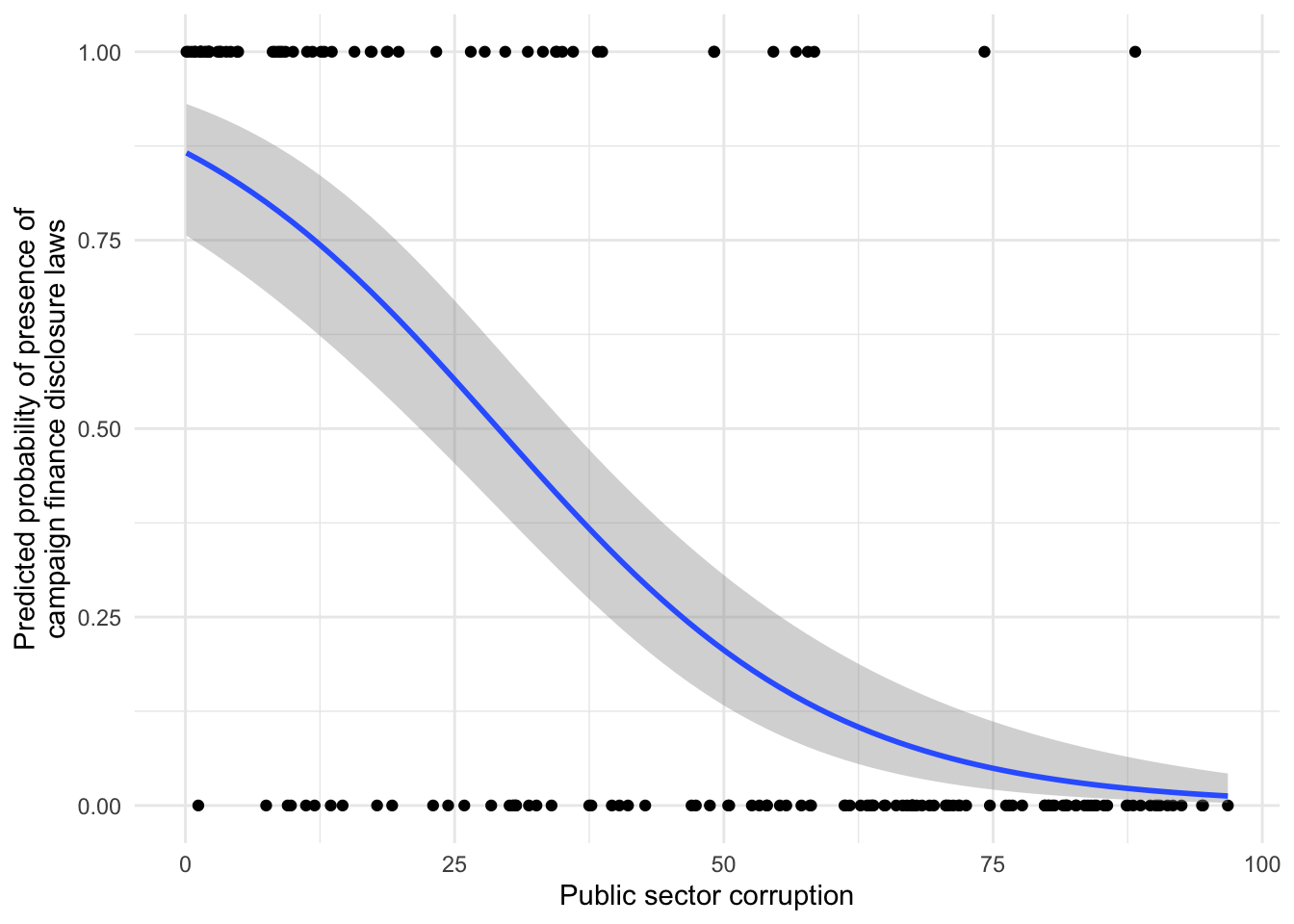
Demo: Estimate a logistic regression model of the effect of public sector corruption on the presence of campaign finance disclosure laws.
# visualize the model
ggplot(
  data = corruption,
  mapping = aes(x = public_sector_corruption, y = as.numeric(disclose_donations))
) +
  geom_point() +
  geom_smooth(method = "glm", method.args = list(family = binomial(link = "logit"))) +
  labs(
    x = "Public sector corruption",
    y = "Predicted probability of presence of\ncampaign finance disclosure laws"
  )
# estimate the model
model_logit <- logistic_reg() |>
  fit(factor(disclose_donations) ~ public_sector_corruption,
    data = corruption
  ) |>
  extract_fit_engine()
tidy(model_logit)
# A tibble: 2 × 5
term estimate std.error statistic p.value
<chr> <dbl> <dbl> <dbl> <dbl>
1 (Intercept) 1.87 0.375 4.99 6.10e- 7
2 public_sector_corruption -0.0644 0.00935 -6.88 5.81e-12Your turn: Interpret the results. What do we learn from this model in terms of the strength and directionality of the relationship? Add response here.
As public sector corruption increases, the predicted probability of the presence of campaign finance disclosure laws decreases. The relationship is negative and relatively strong. Since it is a logistic regression model, the predicted probability curve is not linear and the marginal effect varies depending on the level of public sector corruption.
Potential marginal effects
Your turn: Estimate the average marginal effect and marginal effect at the mean for the logistic regression model. How do the results differ?
# AME
model_logit |>
  avg_slopes()
                     Term Estimate Std. Error     z Pr(>|z|)     S    2.5 %
 public_sector_corruption -0.00816   0.000253 -32.3   <0.001 757.4 -0.00866
   97.5 %
 -0.00767

Columns: term, estimate, std.error, statistic, p.value, s.value, conf.low, conf.high
Type:  response
# ME at the mean
model_logit |>
avg_slopes(newdata = "mean")
                     Term Estimate Std. Error     z Pr(>|z|)    S   2.5 %
 public_sector_corruption   -0.012    0.00163 -7.35   <0.001 42.2 -0.0152
   97.5 %
 -0.00879

Columns: rowid, term, estimate, std.error, statistic, p.value, s.value, conf.low, conf.high, predicted_lo, predicted_hi, predicted
Type:  response
# how do they differ?
bind_rows(
AME = model_logit |>
avg_slopes(),
MEM = model_logit |>
avg_slopes(newdata = "mean"),
.id = "type"
) |>
mutate(type = fct_rev(type)) |>
ggplot(mapping = aes(x = estimate, y = type, color = type)) +
geom_vline(xintercept = 0, linetype = "dashed") +
geom_pointrange(mapping = aes(xmin = conf.low, xmax = conf.high)) +
scale_x_continuous(labels = label_percent()) +
scale_color_discrete_qualitative(guide = "none") +
labs(
x = "Marginal effect (percentage points)",
y = NULL
)
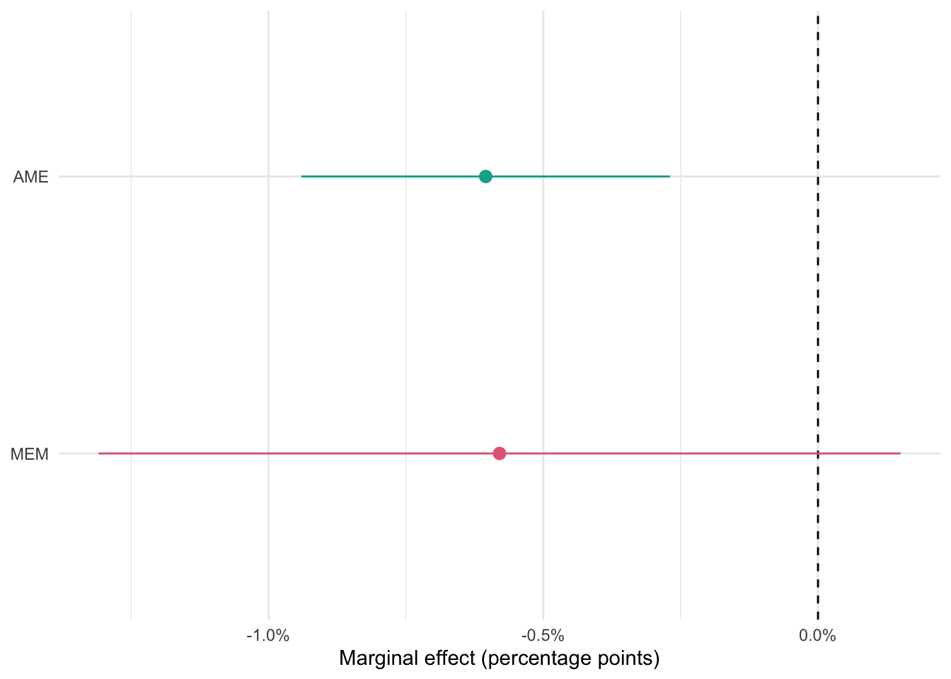
Add response here. The AME is the average marginal effect of public sector corruption on the presence of campaign finance disclosure laws. Here it is \(-0.8\%\) with a relatively compact 95% CI.
The MEM is the marginal effect of public sector corruption on the presence of campaign finance disclosure laws for a country with an average public sector corruption score. Here it is \(-1.2\%\) and the 95% CI is much wider compared to the AME.
Even more complex model
Demo: Estimate a more complex (and potentially realistic) logistic regression model of multiple factors on the presence of campaign finance disclosure laws.
model_logit_fancy <- logistic_reg() |>
  fit(
    factor(disclose_donations) ~ public_sector_corruption + I(public_sector_corruption^2) +
      polyarchy + log_gdp_percapita + public_sector_corruption * region,
    data = corruption
  ) |>
  extract_fit_engine()

# tidied results
tidy(model_logit_fancy)
# A tibble: 15 × 5
term estimate std.error statistic p.value
<chr> <dbl> <dbl> <dbl> <dbl>
1 (Intercept) -4.56e-1 3.70 -0.123 0.902
2 public_sector_corruption -4.22e-2 0.0538 -0.783 0.433
3 I(public_sector_corruption^2) -5.83e-5 0.000548 -0.106 0.915
4 polyarchy 3.43e-2 0.0167 2.06 0.0398
5 log_gdp_percapita 6.09e-2 0.334 0.182 0.855
6 regionLatin America and the Caribbean -2.68e+0 1.50 -1.78 0.0748
7 regionMiddle East and North Africa 9.24e-1 2.41 0.383 0.702
8 regionSub-Saharan Africa -1.69e+0 1.53 -1.10 0.269
9 regionWestern Europe and North America -2.38e-1 1.83 -0.130 0.897
10 regionAsia and Pacific 6.14e-1 1.91 0.321 0.748
11 public_sector_corruption:regionLatin Am… 2.98e-2 0.0329 0.906 0.365
12 public_sector_corruption:regionMiddle E… -4.92e-2 0.0636 -0.774 0.439
13 public_sector_corruption:regionSub-Saha… 1.30e-2 0.0296 0.438 0.662
14 public_sector_corruption:regionWestern … -8.30e-2 0.0990 -0.838 0.402
15 public_sector_corruption:regionAsia and… -4.45e-2 0.0498 -0.894 0.372 Your turn: When interpreting the results as they relate to public sector corruption, does it matter whether your use the AME or MEM?
# focus on slopes for public sector corruption
bind_rows(
  AME = model_logit_fancy |>
    avg_slopes(),
  MEM = model_logit_fancy |>
    avg_slopes(newdata = "mean"),
  .id = "type"
) |>
  filter(term == "public_sector_corruption") |>
  mutate(type = fct_rev(type)) |>
  ggplot(mapping = aes(x = estimate, y = type, color = type)) +
  geom_vline(xintercept = 0, linetype = "dashed") +
  geom_pointrange(mapping = aes(xmin = conf.low, xmax = conf.high)) +
  scale_x_continuous(labels = label_percent()) +
  scale_color_discrete_qualitative(guide = "none") +
  labs(
    x = "Marginal effect (percentage points)",
    y = NULL
  )
Add response here. In certain instances, yes. For the single-variable logistic model there was a substantial difference. However for the more complex model the difference is less pronounced. The point estimates are almost identical, but the MEM has a substantially wider 95% CI that includes 0 compared to the AME.
Group average marginal effects
Your turn: Calculate the average marginal effect of public sector corruption on the presence of campaign finance disclosure laws by region. How does the AME differ by region?
model_logit_fancy |>
  avg_slopes(
    variables = "public_sector_corruption",
    newdata = datagrid(region = levels(corruption$region)),
    by = "region"
  ) |>
  mutate(region = fct_reorder(.f = region, .x = estimate)) |>
  ggplot(mapping = aes(x = estimate, y = region, color = region)) +
  geom_vline(xintercept = 0, linetype = "dashed") +
  geom_pointrange(mapping = aes(xmin = conf.low, xmax = conf.high)) +
  scale_x_continuous(labels = label_percent()) +
  scale_color_discrete_qualitative(guide = "none") +
  labs(
    x = "Marginal effect (percentage points)",
    y = NULL
  )
Add response here. The estimated AME differs across the regions, and only two regions have 95% CIs that do not include 0.
Marginal effects at user-specified or representative values
Demo: Let’s examine countries in three regions (Western Europe, Latin America, and the Middle East) with public sector corruption of 20 and 80. Leave all other values at their typical average.
# create a grid of values
regions_to_use <- c(
  "Western Europe and North America",
  "Latin America and the Caribbean",
  "Middle East and North Africa"
)

# lots of instantaneous marginal effects
model_logit_fancy |>
  slopes(
    variables = "public_sector_corruption",
    newdata = datagrid(
      public_sector_corruption = c(20, 80),
      region = regions_to_use
    )
  )
                     Term public_sector_corruption
 public_sector_corruption                       20
 public_sector_corruption                       20
 public_sector_corruption                       20
 public_sector_corruption                       80
 public_sector_corruption                       80
 public_sector_corruption                       80
                           region  Estimate Std. Error      z Pr(>|z|)   S
 Western Europe and North America -2.62e-02   0.015428 -1.698   0.0896 3.5
 Latin America and the Caribbean  -2.78e-03   0.006462 -0.430   0.6670 0.6
 Middle East and North Africa     -1.90e-02   0.010674 -1.776   0.0757 3.7
 Western Europe and North America -2.11e-05   0.000126 -0.167   0.8671 0.2
 Latin America and the Caribbean  -1.99e-03   0.003390 -0.587   0.5575 0.8
 Middle East and North Africa     -7.41e-04   0.001840 -0.403   0.6871 0.5
     2.5 %   97.5 %
 -0.056429 0.004048
 -0.015446 0.009885
 -0.039881 0.001959
 -0.000269 0.000226
 -0.008633 0.004656
 -0.004347 0.002865

Columns: rowid, term, estimate, std.error, statistic, p.value, s.value, conf.low, conf.high, public_sector_corruption, region, predicted_lo, predicted_hi, predicted, polyarchy, log_gdp_percapita, disclose_donations
Type:  response
Let’s make this more useful. Let’s still focus on the effect of public sector corruption conditional on region, but now visualize across a range of possible values on the \(x\)-axis while holding the other values constant.
# without CIs
plot_predictions(model_logit_fancy, condition = c("public_sector_corruption", "region"), vcov = FALSE) +
  scale_y_continuous(labels = label_percent()) +
  scale_color_discrete_qualitative() +
  labs(
    x = "Public sector corruption",
    y = "Predicted probability of having\na campaign finance disclosure law",
    color = NULL
  ) +
  theme(
    legend.position = "bottom"
  )
# with CIs
plot_predictions(model_logit_fancy, condition = c("public_sector_corruption", "region")) +
  scale_y_continuous(labels = label_percent()) +
  scale_color_discrete_qualitative(aesthetic = c("fill", "color"), guide = "none") +
  facet_wrap(facets = vars(region)) +
  labs(
    x = "Public sector corruption",
    y = "Predicted probability of having\na campaign finance disclosure law",
    color = NULL
  )
Your turn: How do the predicted probabilities vary across region? What do the confidence intervals tell us about this story?
Add response here.
The predicted probabilities appear to differ substantially across the regions based on the different contours of the probability curves. However the 95% CIs reveals that none of the marginal effects are statistically significant. The 95% CIs are so wide it is impossible to determine with certainty what the true relationship is between public sector corruption, region, and the presence of campaign finance disclosure laws.
Acknowledgments
- Application exercise drawn from Marginalia: A guide to figuring out what the heck marginal effects, marginal slopes, average marginal effects, marginal effects at the mean, and all these other marginal things are by Andrew Heiss and licensed under a Creative Commons Attribution 4.0 International License.
Session information
sessioninfo::session_info()─ Session info ───────────────────────────────────────────────────────────────
setting value
version R version 4.3.2 (2023-10-31)
os macOS Ventura 13.6.6
system aarch64, darwin20
ui X11
language (EN)
collate en_US.UTF-8
ctype en_US.UTF-8
tz America/New_York
date 2024-05-01
pandoc 3.1.1 @ /Applications/RStudio.app/Contents/Resources/app/quarto/bin/tools/ (via rmarkdown)
─ Packages ───────────────────────────────────────────────────────────────────
package * version date (UTC) lib source
backports 1.4.1 2021-12-13 [1] CRAN (R 4.3.0)
broom * 1.0.5 2023-06-09 [1] CRAN (R 4.3.0)
checkmate 2.3.1 2023-12-04 [1] CRAN (R 4.3.1)
class 7.3-22 2023-05-03 [1] CRAN (R 4.3.2)
cli 3.6.2 2023-12-11 [1] CRAN (R 4.3.1)
codetools 0.2-19 2023-02-01 [1] CRAN (R 4.3.2)
colorspace * 2.1-0 2023-01-23 [1] CRAN (R 4.3.0)
data.table 1.15.4 2024-03-30 [1] CRAN (R 4.3.1)
dials * 1.2.1 2024-02-22 [1] CRAN (R 4.3.1)
DiceDesign 1.10 2023-12-07 [1] CRAN (R 4.3.1)
digest 0.6.35 2024-03-11 [1] CRAN (R 4.3.1)
dplyr * 1.1.4 2023-11-17 [1] CRAN (R 4.3.1)
evaluate 0.23 2023-11-01 [1] CRAN (R 4.3.1)
fansi 1.0.6 2023-12-08 [1] CRAN (R 4.3.1)
farver 2.1.1 2022-07-06 [1] CRAN (R 4.3.0)
fastmap 1.1.1 2023-02-24 [1] CRAN (R 4.3.0)
forcats * 1.0.0 2023-01-29 [1] CRAN (R 4.3.0)
foreach 1.5.2 2022-02-02 [1] CRAN (R 4.3.0)
furrr 0.3.1 2022-08-15 [1] CRAN (R 4.3.0)
future 1.33.2 2024-03-26 [1] CRAN (R 4.3.1)
future.apply 1.11.2 2024-03-28 [1] CRAN (R 4.3.1)
generics 0.1.3 2022-07-05 [1] CRAN (R 4.3.0)
ggplot2 * 3.5.1 2024-04-23 [1] CRAN (R 4.3.1)
globals 0.16.3 2024-03-08 [1] CRAN (R 4.3.1)
glue 1.7.0 2024-01-09 [1] CRAN (R 4.3.1)
gower 1.0.1 2022-12-22 [1] CRAN (R 4.3.0)
GPfit 1.0-8 2019-02-08 [1] CRAN (R 4.3.0)
gtable 0.3.5 2024-04-22 [1] CRAN (R 4.3.1)
hardhat 1.3.1 2024-02-02 [1] CRAN (R 4.3.1)
here 1.0.1 2020-12-13 [1] CRAN (R 4.3.0)
hms 1.1.3 2023-03-21 [1] CRAN (R 4.3.0)
htmltools 0.5.8.1 2024-04-04 [1] CRAN (R 4.3.1)
htmlwidgets 1.6.4 2023-12-06 [1] CRAN (R 4.3.1)
infer * 1.0.7 2024-03-25 [1] CRAN (R 4.3.1)
insight 0.19.10 2024-03-22 [1] CRAN (R 4.3.1)
ipred 0.9-14 2023-03-09 [1] CRAN (R 4.3.0)
iterators 1.0.14 2022-02-05 [1] CRAN (R 4.3.0)
jsonlite 1.8.8 2023-12-04 [1] CRAN (R 4.3.1)
knitr 1.45 2023-10-30 [1] CRAN (R 4.3.1)
labeling 0.4.3 2023-08-29 [1] CRAN (R 4.3.0)
lattice 0.21-9 2023-10-01 [1] CRAN (R 4.3.2)
lava 1.8.0 2024-03-05 [1] CRAN (R 4.3.1)
lhs 1.1.6 2022-12-17 [1] CRAN (R 4.3.0)
lifecycle 1.0.4 2023-11-07 [1] CRAN (R 4.3.1)
listenv 0.9.1 2024-01-29 [1] CRAN (R 4.3.1)
lubridate * 1.9.3 2023-09-27 [1] CRAN (R 4.3.1)
magrittr 2.0.3 2022-03-30 [1] CRAN (R 4.3.0)
marginaleffects * 0.19.0 2024-04-13 [1] CRAN (R 4.3.1)
MASS 7.3-60 2023-05-04 [1] CRAN (R 4.3.2)
Matrix 1.6-1.1 2023-09-18 [1] CRAN (R 4.3.2)
mgcv 1.9-0 2023-07-11 [1] CRAN (R 4.3.2)
modeldata * 1.3.0 2024-01-21 [1] CRAN (R 4.3.1)
munsell 0.5.1 2024-04-01 [1] CRAN (R 4.3.1)
nlme 3.1-163 2023-08-09 [1] CRAN (R 4.3.2)
nnet 7.3-19 2023-05-03 [1] CRAN (R 4.3.2)
parallelly 1.37.1 2024-02-29 [1] CRAN (R 4.3.1)
parsnip * 1.2.1 2024-03-22 [1] CRAN (R 4.3.1)
pillar 1.9.0 2023-03-22 [1] CRAN (R 4.3.0)
pkgconfig 2.0.3 2019-09-22 [1] CRAN (R 4.3.0)
prodlim 2023.08.28 2023-08-28 [1] CRAN (R 4.3.0)
purrr * 1.0.2 2023-08-10 [1] CRAN (R 4.3.0)
R6 2.5.1 2021-08-19 [1] CRAN (R 4.3.0)
Rcpp 1.0.12 2024-01-09 [1] CRAN (R 4.3.1)
readr * 2.1.5 2024-01-10 [1] CRAN (R 4.3.1)
recipes * 1.0.10 2024-02-18 [1] CRAN (R 4.3.1)
rlang 1.1.3 2024-01-10 [1] CRAN (R 4.3.1)
rmarkdown 2.26 2024-03-05 [1] CRAN (R 4.3.1)
rpart 4.1.21 2023-10-09 [1] CRAN (R 4.3.2)
rprojroot 2.0.4 2023-11-05 [1] CRAN (R 4.3.1)
rsample * 1.2.1 2024-03-25 [1] CRAN (R 4.3.1)
rstudioapi 0.16.0 2024-03-24 [1] CRAN (R 4.3.1)
scales * 1.3.0 2023-11-28 [1] CRAN (R 4.3.1)
sessioninfo 1.2.2 2021-12-06 [1] CRAN (R 4.3.0)
stringi 1.8.3 2023-12-11 [1] CRAN (R 4.3.1)
stringr * 1.5.1 2023-11-14 [1] CRAN (R 4.3.1)
survival 3.5-7 2023-08-14 [1] CRAN (R 4.3.2)
tibble * 3.2.1 2023-03-20 [1] CRAN (R 4.3.0)
tidymodels * 1.2.0 2024-03-25 [1] CRAN (R 4.3.1)
tidyr * 1.3.1 2024-01-24 [1] CRAN (R 4.3.1)
tidyselect 1.2.1 2024-03-11 [1] CRAN (R 4.3.1)
tidyverse * 2.0.0 2023-02-22 [1] CRAN (R 4.3.0)
timechange 0.3.0 2024-01-18 [1] CRAN (R 4.3.1)
timeDate 4032.109 2023-12-14 [1] CRAN (R 4.3.1)
tune * 1.2.1 2024-04-18 [1] CRAN (R 4.3.1)
tzdb 0.4.0 2023-05-12 [1] CRAN (R 4.3.0)
utf8 1.2.4 2023-10-22 [1] CRAN (R 4.3.1)
vctrs 0.6.5 2023-12-01 [1] CRAN (R 4.3.1)
withr 3.0.0 2024-01-16 [1] CRAN (R 4.3.1)
workflows * 1.1.4 2024-02-19 [1] CRAN (R 4.3.1)
workflowsets * 1.1.0 2024-03-21 [1] CRAN (R 4.3.1)
xfun 0.43 2024-03-25 [1] CRAN (R 4.3.1)
yaml 2.3.8 2023-12-11 [1] CRAN (R 4.3.1)
yardstick * 1.3.1 2024-03-21 [1] CRAN (R 4.3.1)
[1] /Library/Frameworks/R.framework/Versions/4.3-arm64/Resources/library
──────────────────────────────────────────────────────────────────────────────