AE 03: Practicing a bunch of geoms
Suggested answers
These are suggested answers. This document should be used as reference only, it’s not designed to be an exhaustive key.
For the following exercises we will work with data on houses that were sold in Tompkins County, NY in 2022-24.1
The variables include:
-
sold_date- date of last recorded sale -
price- sale price (in dollars) -
beds- number of bedrooms -
baths- number of bathrooms. Full bathrooms with shower/toilet count as 1, bathrooms with just a toilet count as 0.5. -
area- living area of the home (in square feet) -
lot_size- size of property’s lot (in acres) -
year_built- year home was built -
hoa_month- monthly HOA dues. If the property is not part of an HOA, then the value isNA -
town- Census-defined town in which the house is located. -
municipality- Census-defined municipality in which the house is located. If the house is located outside of city or village limits, it is classified as “Unincorporated” -
longandlat- geographic coordinates of house
The dataset can be found in the data folder of your repo. It is called tompkins-home-sales.csv. We will import the data and create a new variable, decade_built_cat, which identifies the decade in which the home was built. It will include catch-all categories for any homes pre-1940 and post-1990.
Part 1
Let’s start by visualizing the distribution of the number of bedrooms in the properties sold in Tompkins County, NY in 2022-24. To simplify the task, let’s collapse the variable beds into a smaller number of categories and drop rows with missing values for this variable.
tompkins_beds <- tompkins |>
  mutate(
    beds = factor(beds) |>
      fct_collapse(
        "5+" = c("5", "6", "7", "11")
      )
  ) |>
  drop_na(beds)
Since the number of bedrooms is effectively a categorical variable, we should select a geom appropriate for a single categorical variable.
Your turn: Create a bar chart visualizing the distribution of the number of bedrooms in the properties sold in Tompkins County, NY in 2022-24.

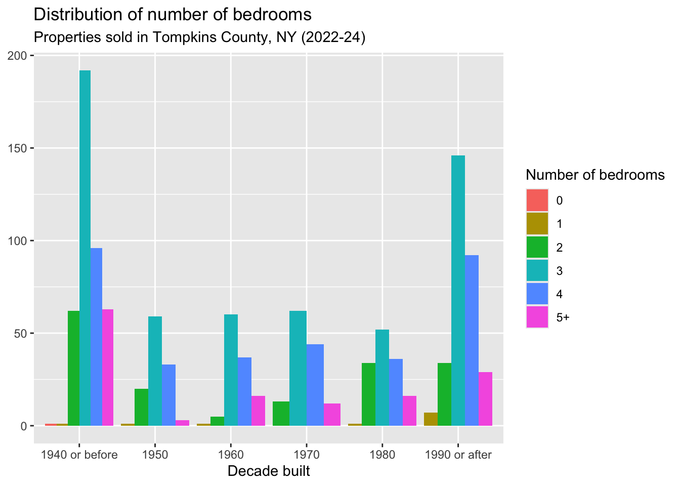
Now let’s visualize the distribution of the number of bedrooms by the decade in which the property was built. We will still use a bar chart but also color-code the bar segments for each decade. Now we have a few variations to consider.
- Stacked bar chart - each bar segment represents the frequency count and are stacked vertically on top of each other.2
- Dodged bar chart - each bar segment represents the frequency count and are placed side by side for each decade. This leaves each segment with a common origin, or baseline value of 0.
- Relative frequency bar chart - each bar segment represents the relative frequency (proportion) of each category within each decade.
Your turn: Generate each form of the bar chart and compare the differences. Which one do you think is the most informative?
Read the documentation for geom_bar() to identify an appropriate argument for specifying each type of bar chart.
ggplot(data = tompkins_beds, mapping = aes(x = decade_built_cat, fill = beds)) +
  # default position is "stack"
  geom_bar(position = "stack") +
  labs(
    title = "Distribution of number of bedrooms",
    subtitle = "Properties sold in Tompkins County, NY (2022-24)",
    x = "Decade built",
    y = NULL,
    fill = "Number of bedrooms"
  )

Part 2
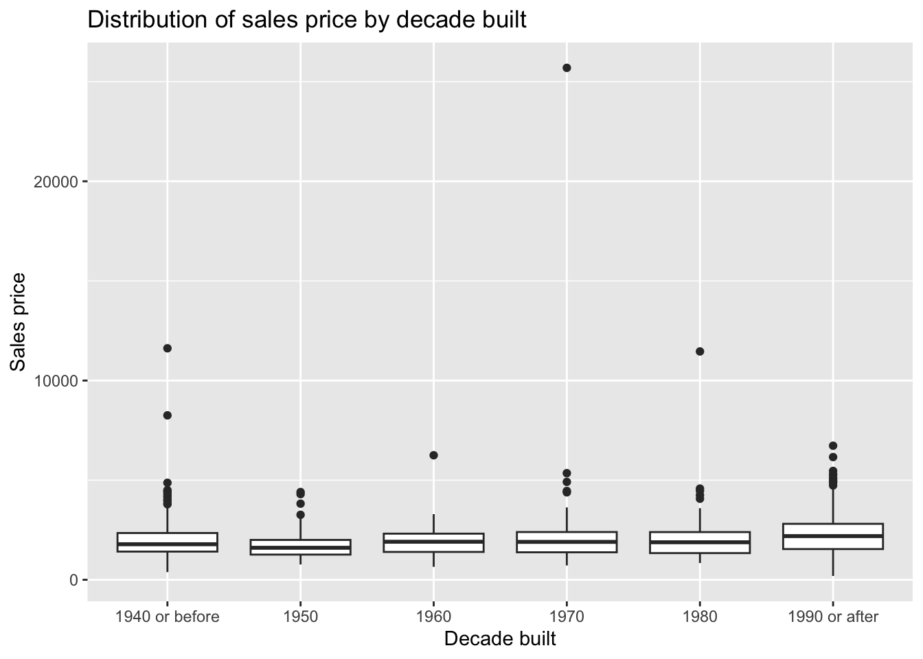
Now let’s evaluate the typical sales price (price) by the decade in which the property was built. We will start by summarizing the data and then visualize the results using a bar chart and a boxplot.
Your turn: Visualize the sales price by the decade in which the property was built. Construct a bar chart reporting the average sales price, as well as a boxplot, violin plot, and strip chart (e.g. jittered scatterplot). What does each graph tell you about the distribution of sales price by decade built? Which ones do you find to be more or less effective?

ggplot(data = tompkins, mapping = aes(x = decade_built_cat, y = area)) +
  geom_boxplot() +
  labs(
    title = "Distribution of sales price by decade built",
    x = "Decade built",
    y = "Sales price"
  )
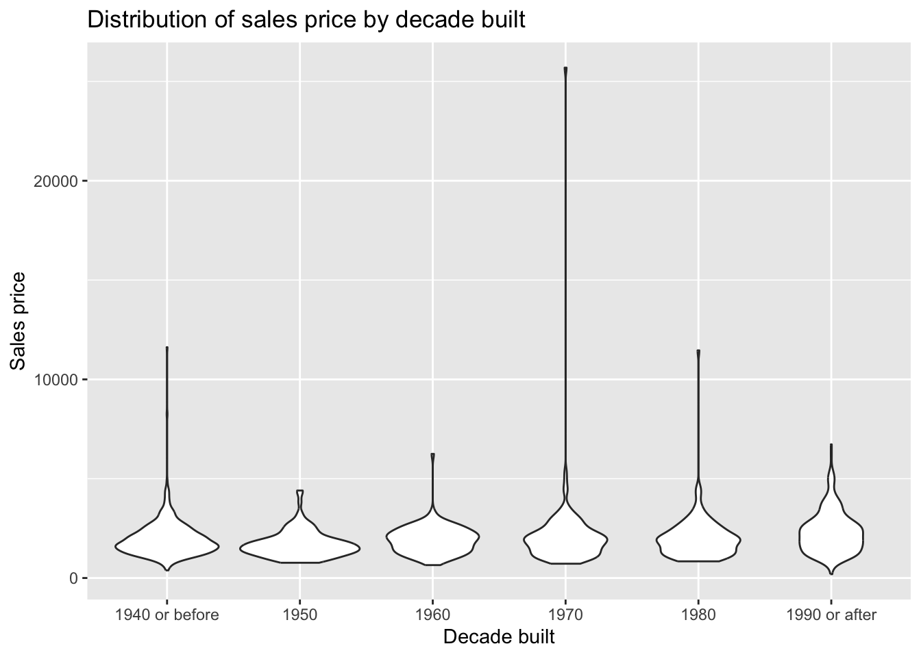
ggplot(data = tompkins, mapping = aes(x = decade_built_cat, y = area)) +
  geom_violin() +
  labs(
    title = "Distribution of sales price by decade built",
    x = "Decade built",
    y = "Sales price"
  )
set.seed(123) # for reproducibility
ggplot(data = tompkins, mapping = aes(x = decade_built_cat, y = area)) +
  geom_jitter(alpha = 0.3) +
  labs(
    title = "Distribution of sales price by decade built",
    x = "Decade built",
    y = "Sales price"
  )
sessioninfo::session_info()─ Session info ───────────────────────────────────────────────────────────────
setting value
version R version 4.5.2 (2025-10-31)
os macOS Tahoe 26.2
system aarch64, darwin20
ui X11
language (EN)
collate C.UTF-8
ctype C.UTF-8
tz America/New_York
date 2026-01-30
pandoc 3.6.3 @ /Applications/Positron.app/Contents/Resources/app/quarto/bin/tools/aarch64/ (via rmarkdown)
quarto 1.9.17 @ /Applications/quarto/bin/quarto
─ Packages ───────────────────────────────────────────────────────────────────
! package * version date (UTC) lib source
P bit 4.6.0 2025-03-06 [?] RSPM (R 4.5.0)
P bit64 4.6.0-1 2025-01-16 [?] RSPM (R 4.5.0)
P cli 3.6.5 2025-04-23 [?] RSPM (R 4.5.0)
P crayon 1.5.3 2024-06-20 [?] RSPM (R 4.5.0)
P digest 0.6.39 2025-11-19 [?] RSPM (R 4.5.0)
P dplyr * 1.1.4 2023-11-17 [?] RSPM (R 4.5.0)
P evaluate 1.0.5 2025-08-27 [?] RSPM (R 4.5.0)
P farver 2.1.2 2024-05-13 [?] RSPM (R 4.5.0)
P fastmap 1.2.0 2024-05-15 [?] RSPM (R 4.5.0)
P forcats * 1.0.1 2025-09-25 [?] RSPM (R 4.5.0)
P generics 0.1.4 2025-05-09 [?] RSPM (R 4.5.0)
P ggplot2 * 4.0.1 2025-11-14 [?] RSPM (R 4.5.0)
P glue 1.8.0 2024-09-30 [?] RSPM (R 4.5.0)
P gtable 0.3.6 2024-10-25 [?] RSPM (R 4.5.0)
P here 1.0.2 2025-09-15 [?] CRAN (R 4.5.0)
P hms 1.1.4 2025-10-17 [?] RSPM (R 4.5.0)
P htmltools 0.5.9 2025-12-04 [?] RSPM (R 4.5.0)
P htmlwidgets 1.6.4 2023-12-06 [?] RSPM (R 4.5.0)
P jsonlite 2.0.0 2025-03-27 [?] RSPM (R 4.5.0)
P knitr 1.51 2025-12-20 [?] RSPM (R 4.5.0)
P labeling 0.4.3 2023-08-29 [?] RSPM (R 4.5.0)
P lifecycle 1.0.4 2023-11-07 [?] RSPM (R 4.5.0)
P lubridate * 1.9.4 2024-12-08 [?] RSPM (R 4.5.0)
P magrittr 2.0.4 2025-09-12 [?] RSPM (R 4.5.0)
P otel 0.2.0 2025-08-29 [?] RSPM (R 4.5.0)
P pillar 1.11.1 2025-09-17 [?] RSPM (R 4.5.0)
P pkgconfig 2.0.3 2019-09-22 [?] RSPM (R 4.5.0)
P purrr * 1.2.0 2025-11-04 [?] CRAN (R 4.5.0)
P R6 2.6.1 2025-02-15 [?] RSPM (R 4.5.0)
P RColorBrewer 1.1-3 2022-04-03 [?] RSPM (R 4.5.0)
P readr * 2.1.6 2025-11-14 [?] RSPM (R 4.5.0)
renv 1.0.11 2024-10-12 [1] CRAN (R 4.5.2)
P rlang 1.1.6 2025-04-11 [?] RSPM (R 4.5.0)
P rmarkdown 2.30 2025-09-28 [?] RSPM (R 4.5.0)
P rprojroot 2.1.1 2025-08-26 [?] RSPM (R 4.5.0)
P S7 0.2.1 2025-11-14 [?] RSPM (R 4.5.0)
P scales 1.4.0 2025-04-24 [?] RSPM (R 4.5.0)
P sessioninfo 1.2.3 2025-02-05 [?] RSPM (R 4.5.0)
P stringi 1.8.7 2025-03-27 [?] RSPM (R 4.5.0)
P stringr * 1.6.0 2025-11-04 [?] RSPM (R 4.5.0)
P tibble * 3.3.0 2025-06-08 [?] RSPM (R 4.5.0)
P tidyr * 1.3.2 2025-12-19 [?] RSPM (R 4.5.0)
P tidyselect 1.2.1 2024-03-11 [?] RSPM (R 4.5.0)
P tidyverse * 2.0.0 2023-02-22 [?] RSPM (R 4.5.0)
P timechange 0.3.0 2024-01-18 [?] RSPM (R 4.5.0)
P tzdb 0.5.0 2025-03-15 [?] RSPM (R 4.5.0)
P vctrs 0.6.5 2023-12-01 [?] RSPM (R 4.5.0)
P vroom 1.6.7 2025-11-28 [?] RSPM (R 4.5.0)
P withr 3.0.2 2024-10-28 [?] RSPM (R 4.5.0)
P xfun 0.55 2025-12-16 [?] CRAN (R 4.5.2)
P yaml 2.3.12 2025-12-10 [?] RSPM (R 4.5.0)
[1] /Users/bcs88/Projects/info-3312/course-site/renv/library/macos/R-4.5/aarch64-apple-darwin20
[2] /Users/bcs88/Library/Caches/org.R-project.R/R/renv/sandbox/macos/R-4.5/aarch64-apple-darwin20/4cd76b74
* ── Packages attached to the search path.
P ── Loaded and on-disk path mismatch.
──────────────────────────────────────────────────────────────────────────────