---
title: "Nobel Prize Laureates: What We Learned"
format:
html:
toc: true
code-fold: true
embed-resources: true
execute:
warning: false
message: false
---
## Overview
This report collects the results of an exploratory session on the `nobel` dataset (one row per laureate and prize). It looks at three questions:
1. Where were recent physics laureates born?
2. How has the typical age at which laureates receive their prize changed over time?
3. Does that age trend look the same across prize categories?
The data is read from `nobel.csv`, which must sit in the same directory as this file.
```{r setup}
library(ggsql)
library(DBI)
library(duckdb)
library(knitr)
# Load the bundled CSV into an in-memory DuckDB database as the "nobel" table
con <- dbConnect(duckdb::duckdb())
nobel <- read.csv("nobel.csv", stringsAsFactors = FALSE)
dbWriteTable(con, "nobel", nobel, overwrite = TRUE)
```
> **Note:** `{ggsql}` chunks run against their own implicit in-memory DuckDB database, so the chunks below read `nobel.csv` directly by path (aliased as `nobel`). The regular R chunks use the `con` connection created above.
## Physics laureates since 2000
### Who won, year by year
```{r physics-laureates}
physics_by_year <- dbGetQuery(con, "
SELECT award_year,
string_agg(name, ', ' ORDER BY name) AS laureates
FROM nobel
WHERE category = 'Physics' AND award_year >= 2000
GROUP BY award_year
ORDER BY award_year
")
kable(physics_by_year, col.names = c("Award year", "Laureates"))
```
### Birth country of physics laureates
The chart counts physics laureates awarded since 2000 by their birth country (present-day borders). Laureates with no recorded birth country, such as organizations, are excluded.
```{r physics-summary}
physics_country <- dbGetQuery(con, "
SELECT birth_country_now, COUNT(*) AS n
FROM nobel
WHERE category = 'Physics' AND award_year >= 2000 AND birth_country_now IS NOT NULL
GROUP BY birth_country_now
ORDER BY n DESC
")
top_country <- physics_country[1, ]
top_share <- top_country$n / sum(physics_country$n)
```
```{ggsql}
SELECT birth_country_now, COUNT(*) AS n FROM 'nobel.csv' AS nobel WHERE category = 'Physics' AND award_year >= 2000 AND birth_country_now IS NOT NULL GROUP BY birth_country_now
VISUALISE birth_country_now AS x, n AS y
DRAW bar ORDER BY n DESC
SCALE DISCRETE x SETTING reverse => true
PROJECT y, x TO cartesian
LABEL x => 'Birth country (present-day)', y => 'Number of laureates'
```
**What we learned:** Among physics laureates since 2000 with a known birth country, the most common birth country is **`r top_country$birth_country_now`** with `r top_country$n` laureates, about `r sprintf("%.0f%%", 100 * top_share)` of the `r sum(physics_country$n)` counted. In total, `r nrow(physics_country)` different countries are represented.
Caveat: counts are by birth country, not by the country where the research was done (see the `affiliation_country` column for that). Shared prizes also mean that one award year can contribute several laureates.
## Age at award over time
### Rolling 10-year median age, all categories
For each award year from 1910 onward, we take all laureates with a known age who were awarded in that year or the nine years before it, and compute the median age at award. A rolling window smooths out the noise from single years, when only a handful of people receive a prize.
```{r age-summary}
age_roll <- dbGetQuery(con, "
WITH years AS (
SELECT DISTINCT CAST(award_year AS INTEGER) AS yr
FROM nobel WHERE age_at_award IS NOT NULL AND award_year >= 1910
)
SELECT y.yr AS award_year,
quantile_cont(n.age_at_award, 0.5) AS rolling_median_age
FROM years y
JOIN nobel n ON n.age_at_award IS NOT NULL AND n.award_year BETWEEN y.yr - 9 AND y.yr
GROUP BY y.yr
ORDER BY y.yr
")
first_row <- age_roll[1, ]
last_row <- age_roll[nrow(age_roll), ]
```
```{ggsql}
WITH years AS (
SELECT DISTINCT CAST(award_year AS INTEGER) AS yr FROM 'nobel.csv' WHERE age_at_award IS NOT NULL AND award_year >= 1910
)
SELECT y.yr AS award_year,
quantile_cont(n.age_at_award, 0.5) AS rolling_median_age
FROM years y
JOIN 'nobel.csv' n ON n.age_at_award IS NOT NULL AND n.award_year BETWEEN y.yr - 9 AND y.yr
GROUP BY y.yr
ORDER BY y.yr
VISUALISE award_year AS x, rolling_median_age AS y
DRAW line
LABEL x => 'Award year (end of 10-year window)', y => 'Rolling median age at award (years)'
```
**What we learned:** The rolling median age was **`r round(first_row$rolling_median_age, 1)`** years for the window ending in `r first_row$award_year` and **`r round(last_row$rolling_median_age, 1)`** years for the window ending in `r last_row$award_year`. The line shows the path between those two points, so the overall direction and any periods of faster change can be read from the chart.
### Rolling 10-year median age, by category
The same calculation is repeated separately for each prize category. Windows containing fewer than five laureates are dropped so that the medians are not driven by one or two people.
```{ggsql}
WITH cat_years AS (
SELECT DISTINCT category, CAST(award_year AS INTEGER) AS yr
FROM 'nobel.csv' WHERE age_at_award IS NOT NULL
)
SELECT cy.category,
cy.yr AS award_year,
quantile_cont(n.age_at_award, 0.5) AS rolling_median_age
FROM cat_years cy
JOIN 'nobel.csv' n
ON n.category = cy.category
AND n.age_at_award IS NOT NULL
AND n.award_year BETWEEN cy.yr - 9 AND cy.yr
GROUP BY cy.category, cy.yr
HAVING COUNT(*) >= 5 -- skip windows with too few laureates
ORDER BY cy.category, cy.yr
VISUALISE award_year AS x, rolling_median_age AS y
DRAW line
FACET category SETTING ncol => 3
LABEL x => 'Award year (end of 10-year window)', y => 'Rolling median age at award (years)'
```
**What we learned:** Faceting by category shows whether the overall age trend is shared by every prize or driven by a few. Compare the vertical level of each panel (typical age) and its slope (change over time). Categories such as Economic Sciences were introduced later, so their lines start later.
## Summary of findings
- **Geography:** Recent physics laureates come from a small number of countries, with `r top_country$birth_country_now` the most common birth country (`r top_country$n` of `r sum(physics_country$n)` counted laureates).
- **Age overall:** The rolling median age at award moved from `r round(first_row$rolling_median_age, 1)` to `r round(last_row$rolling_median_age, 1)` years between the first and last windows.
- **Age by category:** Categories differ in both their typical age and how it has changed, so the overall trend should not be assumed to hold for each prize.
### Caveats and next steps
- Rolling windows are defined by award year and overlap, so neighbouring points are not independent.
- Birth country reflects present-day borders (`birth_country_now`) and may differ from the country at the time of birth.
- Natural follow-ups: compare affiliation country with birth country, and look at how the number of shared prizes (`n_shared`) relates to laureate age.
```{r cleanup, include=FALSE}
dbDisconnect(con, shutdown = TRUE)
```Generative AI and data visualization
Lecture 21
Dr. Benjamin Soltoff
Cornell University
INFO 3312/5312 - Fall 2026
November 19, 2026
Announcements
Announcements
- Homework 06 due after Thanksgiving Break
- Project 03
Learning objectives
- Evaluate coding assistants for exploratory data analysis
- Create natural language interfaces to data with {querychat}
- Define the workflow of a {querychat} app
- Introduce ggsql for charts
Application exercise
ae-22
Instructions
- Go to the course GitHub org and find your
ae-22(repo name will be suffixed with your GitHub name). - Clone the repo in Positron, run
renv::restore()to install the required packages, open the Quarto document in the repo, and follow along and complete the exercises. - Render, commit, and push your edits by the AE deadline – end of the day
🔓 Decrypt the .Renviron.secret → .Renviron
source("secret.R")- The special phrase is:
info-3312
Reset Posit Assistant to use the new API keys
- Copy your key: run
Sys.getenv("ANTHROPIC_API_KEY")in the console - Open the Posit Assistant pane and choose Configure AI providers (model selector, gear menu, or Command Palette)
- Select Anthropic, paste the key, and save
The impact of generative AI on data visualization
What’s changing
- Coding assistants such as Posit Assistant, Claude Code, and GitHub Copilot write and run analysis code
- People can upload data files to Claude/ChatGPT and ask it questions about the data
- LLMs can build dashboards and data-integrated products on their own
Today’s question
What is the role of the human being in data communication today? What will it be a year from now?
Exploratory data analysis with Posit Assistant
Posit Assistant for EDA
AI harness for human-guided exploratory analysis
Use to generate reproducible code for data cleaning and EDA
- Load the data (either yourself or ask it to do so)
- Enter
/cleanmode to check and clean the data - Exit clean, conduct EDA: ask questions, request plots, and explore patterns
- Run
/eda-logto see what you’ve explored so far - Run
/report(Quarto) or/notebook(Jupyter) to save your findings in a reproducible notebook
Specific questions get better answers
Vague
Show me a histogram.
Specific
Show me the distribution of age at award for each prize category, with the median marked.
Tip
The assistant’s suggestions are only suggestions – you should decide where to go next.
The data: Nobel Prize laureates
Every laureate from 1901 to 2026 from the Nobel Prize API
{
  "knownName": { "en": "Marie Curie", "se": "Marie Curie" },
  "gender": "female",
  "birth": { "date": "1867-11-07", "place": {
      "country": { "en": "Russian Empire", ... },
      "countryNow": { "en": "Poland", ... }, ... } },
  "nobelPrizes": [
    { "awardYear": "1903", "category": { "en": "Physics", ... }, "portion": "1/4", ... },
    { "awardYear": "1911", "category": { "en": "Chemistry", ... }, "portion": "1", ... }
  ]
}
⌨️ Your turn - Explore the Nobel data
Instructions
Use Posit Assistant to get data/nobel-laureates.json into a tidy data frame, explore it, and save your analysis with /report.
Keep track of two things:
- Two or three insights you’d share with someone who knows nothing about the data
- The decisions made along the way. What got kept, dropped, recoded, or summarized? Who made each call, you or the assistant?
12:00
⌨️ Your turn - Explore the Nobel data
Instructions
Discuss with a partner
- Where were you driving, and where were you a passenger?
- Did you clean the data the same way? Did you get the same numbers?
- When did you accept a suggestion without checking it?
- When did you change direction because of something you knew or noticed?
04:00
What does the human bring?
The LLM is good at
- Writing boilerplate code fast
- Parsing awkward formats like nested JSON
- Suggesting directions to explore
- Remembering function names and syntax
You are still responsible for
- Asking questions worth answering
- Choosing how to clean the data, and knowing what each choice changes
- Knowing the domain
- Checking that the numbers are right
- Picking the chart, the design, and the message for your audience
Natural language interfaces with querychat
Not everyone wants an IDE
- Many people who need answers from data don’t write code
- They still need results that someone else can rerun and check
- They want charts, tables, and reports they can keep and share
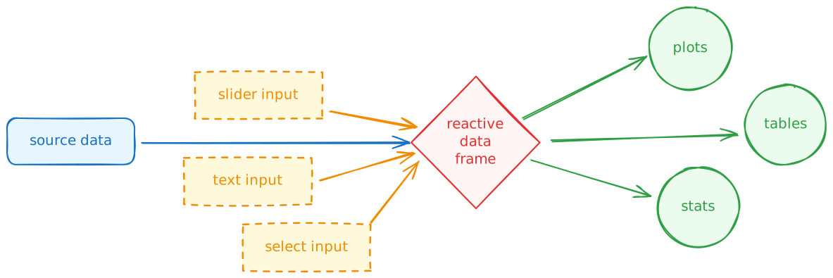
A standard Shiny app
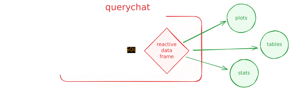
A {querychat} app
{querychat} in R
library(querychat)

nobel <- read_csv(here("data/nobel.csv"))

querychat_app(
  nobel,
  table_name = "nobel",
  client = "anthropic/claude-sonnet-5-5",
  # context for the LLM: what the columns mean and how to use them
  data_description = here("data/nobel-description.md"),
  # shown when the app opens
  greeting = here("data/greeting.md")
)
querychat_app() builds and launches a complete chat app around one dataset.
Beyond the chat app
QueryChat$new() exposes the pieces of the app, so you can build your own dashboard around the chat:
$sidebar()puts the chat in a {bslib} sidebar$server()returnsdf(),sql(), andtitle(), reactives for the filtered data, the SQL behind it, and a short label- You connect those reactives to your own plots, tables, and value boxes
⌨️ Your turn - ex-02 (part 1)
Instructions
Run exercises/ex-02-app.R. Ask one question of each kind:
- Filter. “Show only laureates in Physics since 2000”
- Summarize. “Who was the youngest laureate in each category?”
- Visualize. “Plot the share of female laureates by decade”
Open the tool card under each answer. Which tool was called? What programming language did it write?
05:00
How {querychat} works
Tool calling
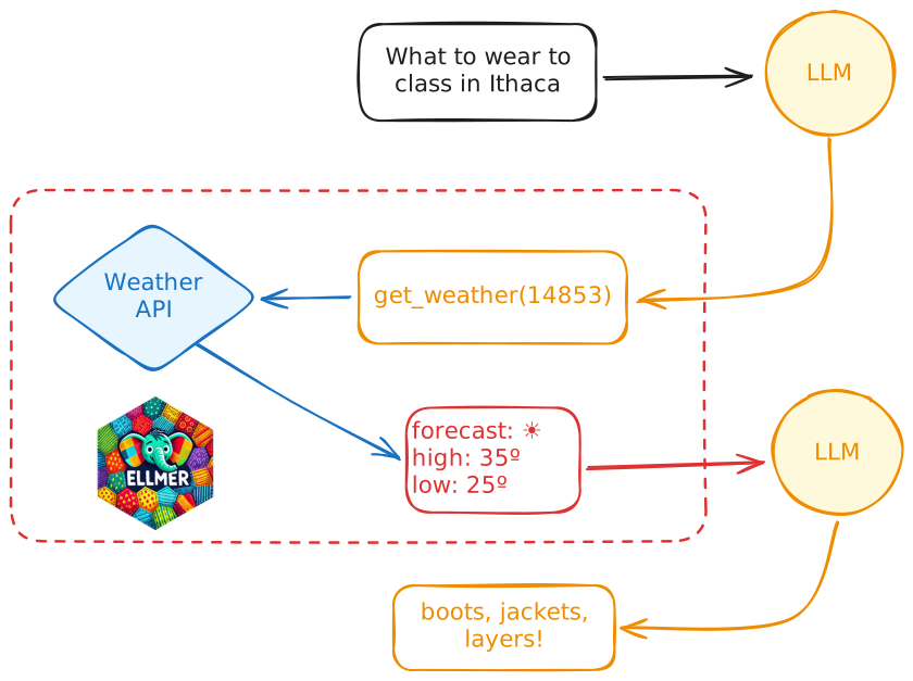
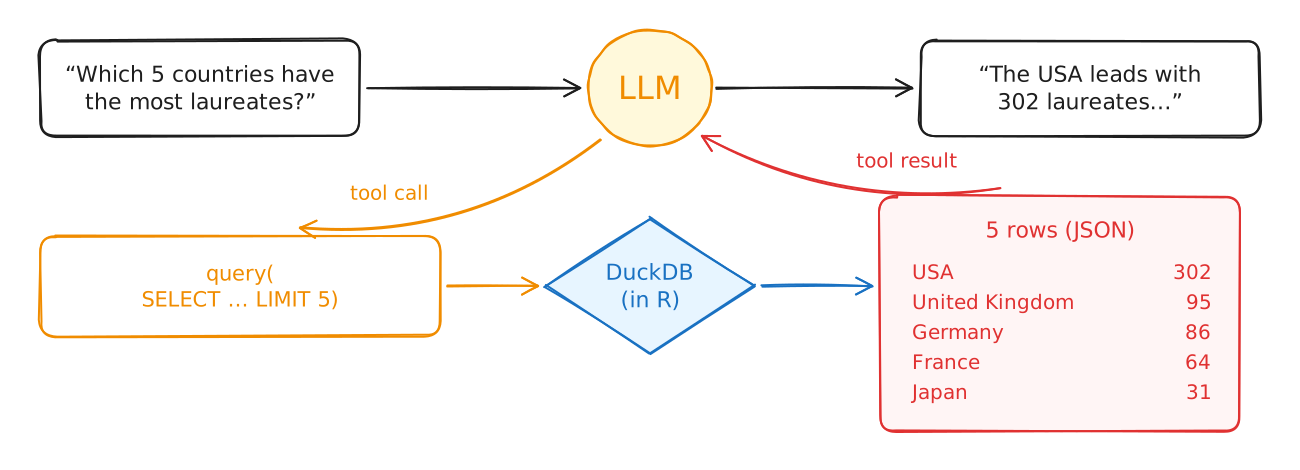
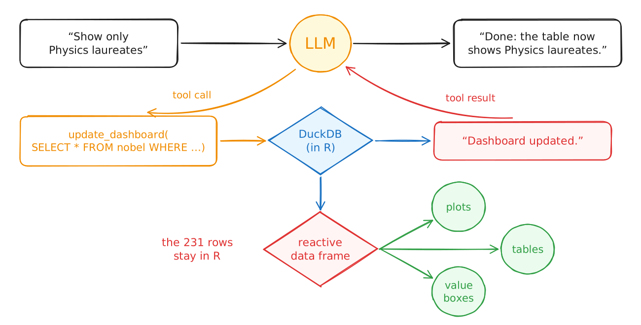
The LLM can’t run code. It asks the app to call a tool, and the app sends back the result.
querychat’s tools
| Tool | Used for | Sent back to the LLM |
|---|---|---|
get_schema |
Learning the table’s structure | Column names, types, ranges, low-cardinality values |
update_dashboard |
“Show me…”, “Filter to…” | Only “Dashboard updated.” |
reset_dashboard |
“Start over” | A confirmation |
query |
“Who…?”, “How many…?” | The result rows |
visualize |
“Plot…” | A PNG image of the chart |
A summary request
A filter request
So does the LLM see my data?
- It never gets the whole table, and it never does the math. DuckDB runs every query on your computer.
- It does see
- Column names, types, and ranges
- Every value of text columns with few distinct values
- Your data description
- The rows returned by every summary query
- A PNG of every chart
- With
tools = "filter"the LLM can only filter the table, so no query results leave your computer
From chat to a reproducible report
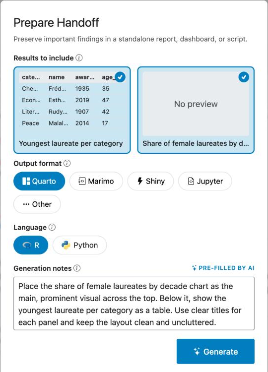
Type /handoff in the chat.
- Select the results you want to keep
- Pick a format (Quarto, Shiny, Jupyter, …)
- The LLM writes the document with the same SQL from your chat
- Download a zip with the document and the data
- Render it yourself
What is in the report
A setup chunk loads the bundled data, {ggsql} chunks redraw your charts, and {r} chunks rerun your summary queries.
⌨️ Your turn - ex-02 (part 2)
Instructions
- Type
/handoff. Select the results you want to keep, choose Quarto and R, and generate. - Download the bundle, unzip it, open the
.qmd, and render it. - Do the numbers and charts match what you saw in the chat? What would you change before sharing it?
06:00
ggsql: a grammar of graphics in SQL
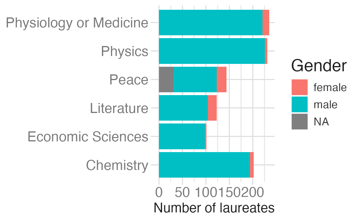
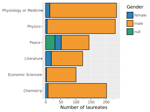
The grammar of graphics in SQL
| {ggplot2} | ggsql |
|---|---|
ggplot(data, aes(...)) |
VISUALISE ... FROM data |
geom_*() |
DRAW layer |
aes() inside a geom |
MAPPING ... AS aesthetic |
scale_*() |
SCALE |
facet_wrap() |
FACET |
coord_*() |
PROJECT |
labs() |
LABEL |
SQL first, then VISUALISE
SELECT FLOOR(award_year / 10) * 10 AS decade,
  100 * AVG(CASE WHEN gender = 'female'
    THEN 1 ELSE 0 END) AS pct_female
FROM r:nobel
WHERE gender IS NOT NULL
GROUP BY decade
VISUALISE decade AS x, pct_female AS y
DRAW line
DRAW point
LABEL title => 'Female Nobel laureates',
  x => 'Decade', y => 'Share of laureates (%)'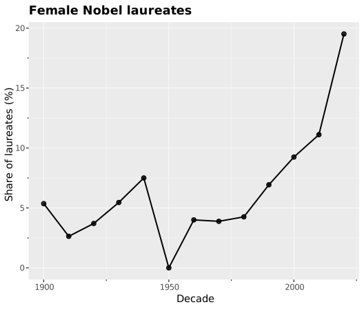
Layers and facets
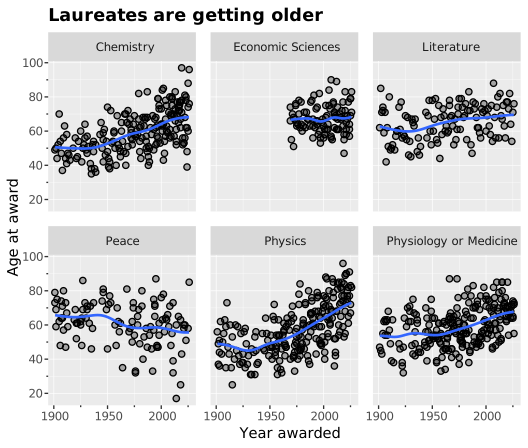
Why give an LLM ggsql instead of {ggplot2}?
- Security
- The app should never run arbitrary R code written by the LLM
- Instead, the LLM writes a declarative query that is run in read-only SQL
- LLMs are already great at writing SQL
- The same query renders in R, Python, Quarto, Jupyter, Shiny, etc.
The tradeoffs
ggsql is young (version 0.5), so expect bugs
It has far fewer layers, scales, and extensions than {ggplot2}
You get less control over themes and annotations
It’s another language to learn, though you already know the grammar
Wrap-up
Recap
- Coding assistants speed up EDA, but you still decide how to clean the data, bring the domain knowledge, and check the results
- {querychat} turns questions into SQL with tool calling, and all SQL runs on your computer
- The LLM sees the schema, your data description, summary query results, and chart images. It never sees the rows behind a filter.
/handoffturns a chat session into a Quarto report you can rerun- ggsql is a grammar of graphics in SQL. An app can let an LLM write ggsql without running the LLM’s code.
Learn more
Acknowledgements
- {querychat} materials derived in part from Programming with LLMs and licensed under a Creative Commons Attribution 4.0 International (CC BY) License.
- Nobel Prize data from the Nobel Prize API.
