# A tibble: 3,370 × 5
   broad_field   major_field                                 field                       year n_phds
   <chr>         <chr>                                       <chr>                      <dbl>  <dbl>
 1 Life sciences Agricultural sciences and natural resources Agricultural economics      2008    111
 2 Life sciences Agricultural sciences and natural resources Agricultural and horticul…  2008     28
 3 Life sciences Agricultural sciences and natural resources Agricultural animal breed…  2008      3
 4 Life sciences Agricultural sciences and natural resources Agronomy and crop science   2008     68
 5 Life sciences Agricultural sciences and natural resources Animal nutrition            2008     41
 6 Life sciences Agricultural sciences and natural resources Animal science, poultry o…  2008     18
 7 Life sciences Agricultural sciences and natural resources Animal sciences, other      2008     77
 8 Life sciences Agricultural sciences and natural resources Environmental science       2008    182
 9 Life sciences Agricultural sciences and natural resources Fishing and fisheries sci…  2008     52
10 Life sciences Agricultural sciences and natural resources Food science                2008     96
# ℹ 3,360 more rowsTables
Lecture 25
April 30, 2024
PhDs awarded in 2017
# A tibble: 7 × 2
  field                               perc
  <chr>                              <dbl>
1 Life sciences                     0.408
2 Mathematics and computer sciences 0.0710
3 Psychology and social sciences    0.236
4 Engineering                       0.0412
5 Education                         0.0891
6 Humanities and arts               0.0978
7 Other                             0.0575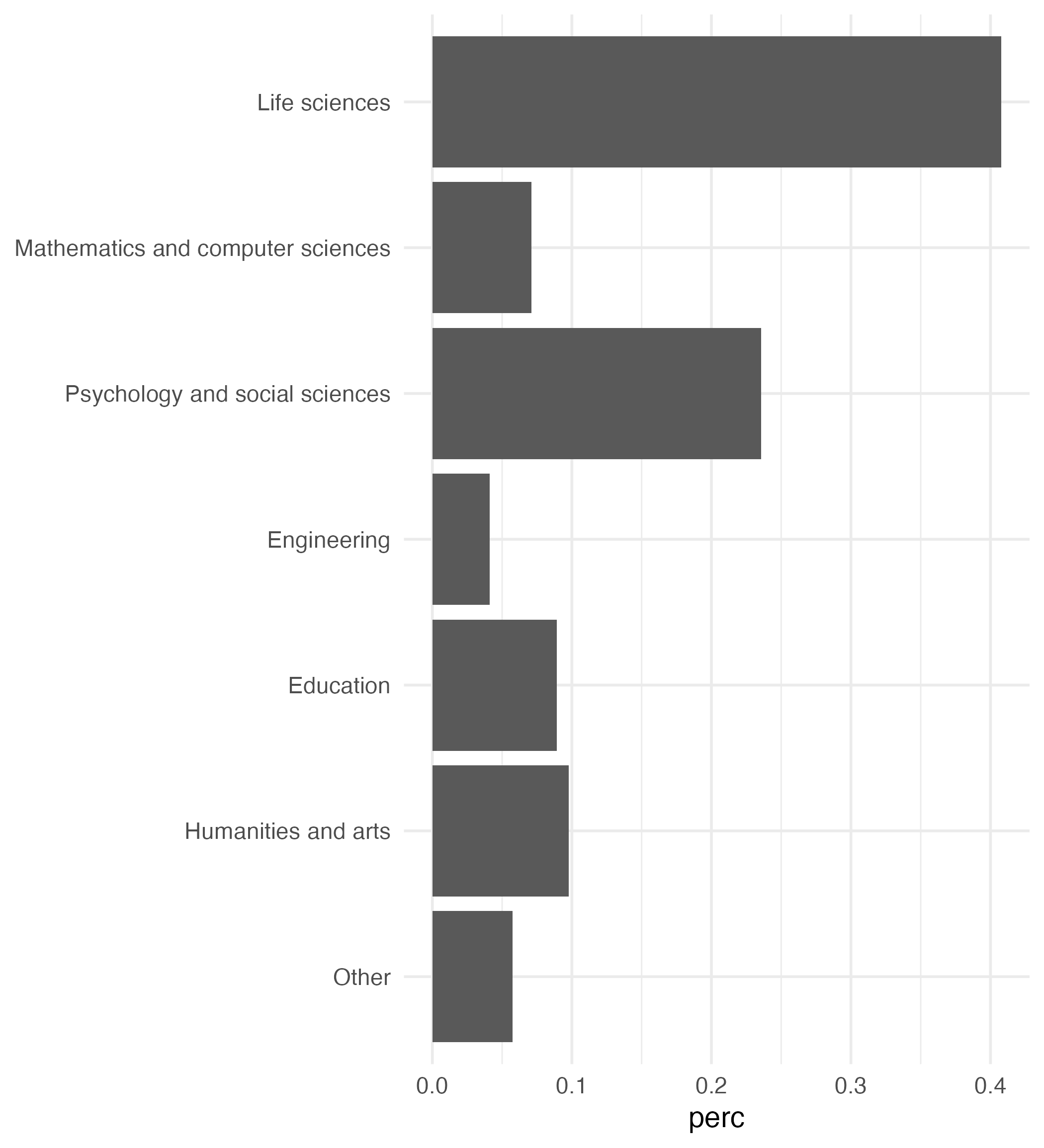
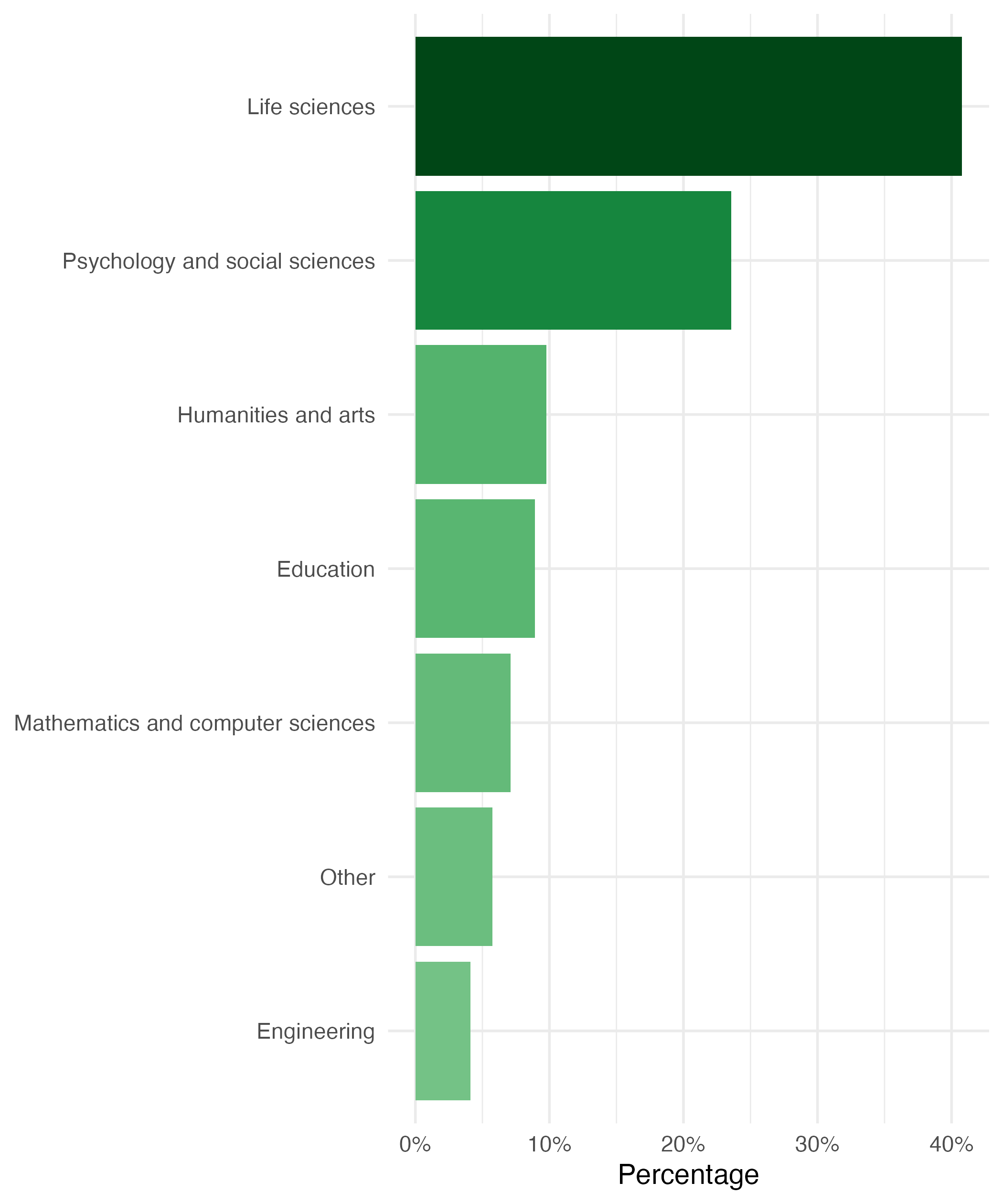
PhDs awarded in 2017
# A tibble: 7 × 2
  field                               perc
  <chr>                              <dbl>
1 Life sciences                     0.408
2 Psychology and social sciences    0.236
3 Humanities and arts               0.0978
4 Education                         0.0891
5 Mathematics and computer sciences 0.0710
6 Other                             0.0575
7 Engineering                       0.0412
PhDs awarded in 2017
| Field | Percentage |
|---|---|
| Life sciences | 40.8% |
| Psychology and social sciences | 23.6% |
| Humanities and arts | 9.8% |
| Education | 8.9% |
| Mathematics and computer sciences | 7.1% |
| Other | 5.8% |
| Engineering | 4.1% |
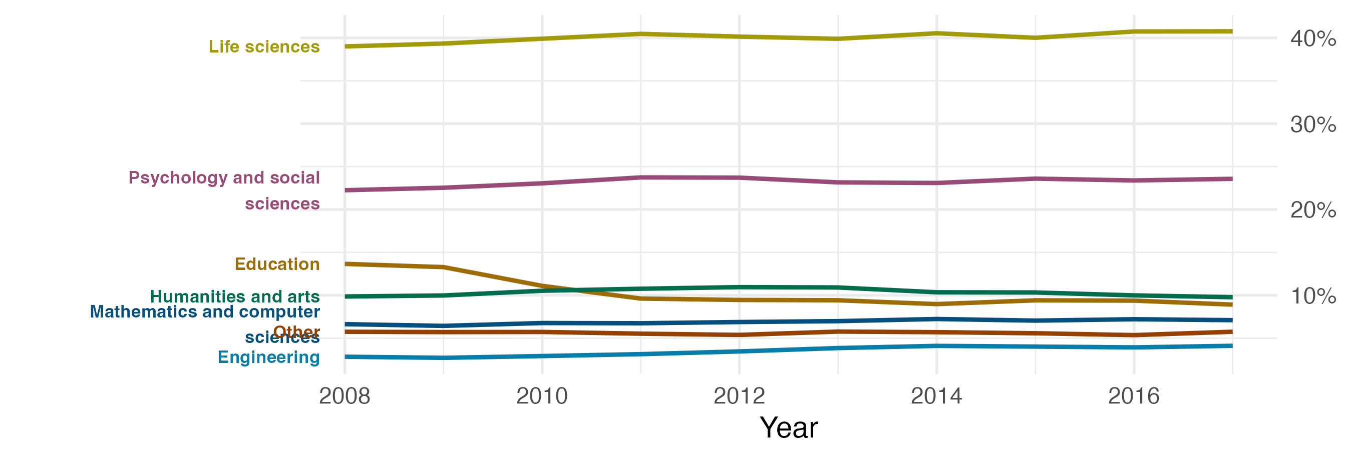
Or in a plot?
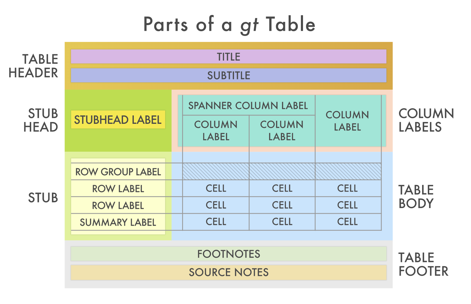
Tables with gt
We will use the gt (Grammar of Tables) package to create tables in R.
The gt philosophy: we can construct a wide variety of useful tables with a cohesive set of table parts.
Source: gt.rstudio.com
Tables with gt

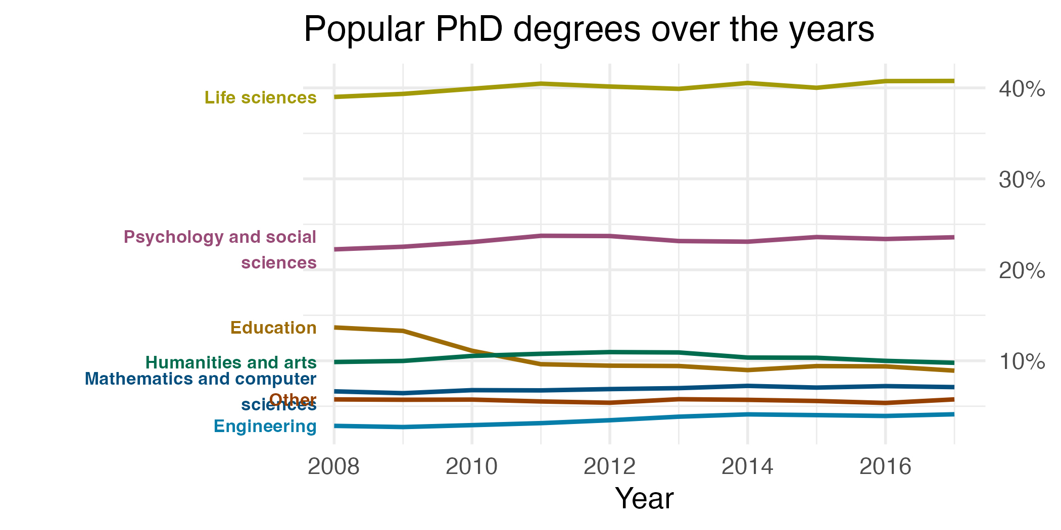
Should these data be displayed in a table or a plot?
Popular PhD degrees over the years
|
||||||||||
|---|---|---|---|---|---|---|---|---|---|---|
| Field | 2008 | 2009 | 2010 | 2011 | 2012 | 2013 | 2014 | 2015 | 2016 | 2017 |
| Life sciences | 39% | 39% | 40% | 40% | 40% | 40% | 41% | 40% | 41% | 41% |
| Mathematics and computer sciences | 7% | 6% | 7% | 7% | 7% | 7% | 7% | 7% | 7% | 7% |
| Psychology and social sciences | 22% | 23% | 23% | 24% | 24% | 23% | 23% | 24% | 23% | 24% |
| Engineering | 3% | 3% | 3% | 3% | 3% | 4% | 4% | 4% | 4% | 4% |
| Education | 14% | 13% | 11% | 10% | 9% | 9% | 9% | 9% | 9% | 9% |
| Humanities and arts | 10% | 10% | 11% | 11% | 11% | 11% | 10% | 10% | 10% | 10% |
| Other | 6% | 6% | 6% | 6% | 5% | 6% | 6% | 6% | 5% | 6% |
Add visualizations to your table
Example: Add sparklines to display trend alongside raw data
Popular Bachelor's degrees over the years
|
|||||||||||
|---|---|---|---|---|---|---|---|---|---|---|---|
| Field | Trend | 2008 | 2009 | 2010 | 2011 | 2012 | 2013 | 2014 | 2015 | 2016 | 2017 |
| Education |  |
14% | 13% | 11% | 10% | 9% | 9% | 9% | 9% | 9% | 9% |
| Engineering |  |
3% | 3% | 3% | 3% | 3% | 4% | 4% | 4% | 4% | 4% |
| Humanities and arts |  |
10% | 10% | 11% | 11% | 11% | 11% | 10% | 10% | 10% | 10% |
| Life sciences |  |
39% | 39% | 40% | 40% | 40% | 40% | 41% | 40% | 41% | 41% |
| Mathematics and computer sciences |  |
7% | 6% | 7% | 7% | 7% | 7% | 7% | 7% | 7% | 7% |
| Other |  |
6% | 6% | 6% | 6% | 5% | 6% | 6% | 6% | 5% | 6% |
| Psychology and social sciences |  |
22% | 23% | 23% | 24% | 24% | 23% | 23% | 24% | 23% | 24% |
Custom function with ggplot()

Basic gt table with sparklines
| field | ggplot | 2008 | 2009 | 2010 | 2011 | 2012 | 2013 | 2014 | 2015 | 2016 | 2017 |
|---|---|---|---|---|---|---|---|---|---|---|---|
| Life sciences |  |
0.39003873 | 0.39339859 | 0.39902998 | 0.40466774 | 0.40148099 | 0.39893069 | 0.40538565 | 0.40009972 | 0.40745871 | 0.40763260 |
| Mathematics and computer sciences |  |
0.06635989 | 0.06436580 | 0.06767028 | 0.06742059 | 0.06885007 | 0.06988734 | 0.07237089 | 0.07050264 | 0.07210820 | 0.07102199 |
| Psychology and social sciences |  |
0.22246283 | 0.22535154 | 0.23049467 | 0.23738310 | 0.23711523 | 0.23160206 | 0.23090473 | 0.23597518 | 0.23384127 | 0.23576049 |
| Engineering |  |
0.02840128 | 0.02712603 | 0.02920551 | 0.03141350 | 0.03460228 | 0.03851442 | 0.04105764 | 0.04021864 | 0.03929860 | 0.04115690 |
| Education |  |
0.13661350 | 0.13284223 | 0.11100613 | 0.09619742 | 0.09459007 | 0.09421424 | 0.08974215 | 0.09413894 | 0.09379899 | 0.08913325 |
| Humanities and arts |  |
0.09861325 | 0.09979447 | 0.10529520 | 0.10765048 | 0.10951809 | 0.10912736 | 0.10351548 | 0.10329800 | 0.09988699 | 0.09776381 |
| Other |  |
0.05751052 | 0.05712134 | 0.05729823 | 0.05526717 | 0.05384328 | 0.05772389 | 0.05702346 | 0.05576689 | 0.05360723 | 0.05753096 |
Generate the table
Popular PhD degrees over the years
|
|||||||||||
|---|---|---|---|---|---|---|---|---|---|---|---|
| Field | Trend | 2008 | 2009 | 2010 | 2011 | 2012 | 2013 | 2014 | 2015 | 2016 | 2017 |
| Life sciences | |
39% | 39% | 40% | 40% | 40% | 40% | 41% | 40% | 41% | 41% |
| Mathematics and computer sciences | |
7% | 6% | 7% | 7% | 7% | 7% | 7% | 7% | 7% | 7% |
| Psychology and social sciences | |
22% | 23% | 23% | 24% | 24% | 23% | 23% | 24% | 23% | 24% |
| Engineering | |
3% | 3% | 3% | 3% | 3% | 4% | 4% | 4% | 4% | 4% |
| Education | |
14% | 13% | 11% | 10% | 9% | 9% | 9% | 9% | 9% | 9% |
| Humanities and arts | |
10% | 10% | 11% | 11% | 11% | 11% | 10% | 10% | 10% | 10% |
| Other | |
6% | 6% | 6% | 6% | 5% | 6% | 6% | 6% | 5% | 6% |
Adding color text
Popular Bachelor's degrees over the years
|
|||||||||||
|---|---|---|---|---|---|---|---|---|---|---|---|
| Field | Trend | 2008 | 2009 | 2010 | 2011 | 2012 | 2013 | 2014 | 2015 | 2016 | 2017 |
| Education | |
14% | 13% | 11% | 10% | 9% | 9% | 9% | 9% | 9% | 9% |
| Engineering | |
3% | 3% | 3% | 3% | 3% | 4% | 4% | 4% | 4% | 4% |
| Humanities and arts | |
10% | 10% | 11% | 11% | 11% | 11% | 10% | 10% | 10% | 10% |
| Life sciences | |
39% | 39% | 40% | 40% | 40% | 40% | 41% | 40% | 41% | 41% |
| Mathematics and computer sciences | |
7% | 6% | 7% | 7% | 7% | 7% | 7% | 7% | 7% | 7% |
| Other | |
6% | 6% | 6% | 6% | 5% | 6% | 6% | 6% | 5% | 6% |
| Psychology and social sciences | |
22% | 23% | 23% | 24% | 24% | 23% | 23% | 24% | 23% | 24% |
plot_spark_color <- function(df) {
  ggplot(df, aes(x = year, y = perc, color = line_color)) +
    geom_line(size = 20) +
    theme_void() +
    scale_color_identity()
}

phd_degrees_other_plots_color <- phd_degrees_other |>
  mutate(line_color = case_when(
    field == "Education" ~ "#9D6C06",
    field == "Engineering" ~ "#077DAA",
    field == "Humanities and arts" ~ "#026D4E",
    field == "Life sciences" ~ "#A39A09",
    field == "Mathematics and computer sciences" ~ "#044F7E",
    field == "Other" ~ "#954000",
    field == "Psychology and social sciences" ~ "#984B77"
  )) |>
  nest(field_df = c(year, perc, line_color)) |>
  mutate(plot = map(field_df, plot_spark_color)) |>
  arrange(field)

phd_degrees_other |>
  pivot_wider(names_from = year, values_from = perc) |>
  arrange(field) |>
  mutate(ggplot = NA, .after = field) |>
  gt() |>
  text_transform(
    locations = cells_body(columns = ggplot),
    fn = \(x) {
      map(phd_degrees_other_plots_color$plot, ggplot_image, height = px(15), aspect_ratio = 4)
    }
  ) |>
  cols_width(ggplot ~ px(100)) |>
  cols_align(align = "left", columns = field) |>
  fmt_percent(columns = where(is.numeric), decimals = 0) |>
  tab_style(style = cell_text(color = "#9D6C06"), locations = cells_body(rows = 1, columns = field)) |>
  tab_style(style = cell_text(color = "#077DAA"), locations = cells_body(rows = 2, columns = field)) |>
  tab_style(style = cell_text(color = "#026D4E"), locations = cells_body(rows = 3, columns = field)) |>
  tab_style(style = cell_text(color = "#A39A09"), locations = cells_body(rows = 4, columns = field)) |>
  tab_style(style = cell_text(color = "#044F7E"), locations = cells_body(rows = 5, columns = field)) |>
  tab_style(style = cell_text(color = "#954000"), locations = cells_body(rows = 6, columns = field)) |>
  tab_style(style = cell_text(color = "#984B77"), locations = cells_body(rows = 7, columns = field)) |>
  cols_label(field = "Field", ggplot = "Trend") |>
  tab_spanner(label = "Popular Bachelor's degrees over the years", columns = everything()) |>
  tab_style(style = cell_text(weight = "bold"), locations = cells_column_spanners())