Explainable machine learning models

Lecture 25

Dr. Benjamin Soltoff

Cornell University
INFO 3312/5312 - Spring 2024

May 4, 2023

Announcements

Presentations tomorrow
Course evaluations – 0.5% extra credit towards your final grade if you complete your course evaluation by May 12

Setup

Packages + figures

# load packages
library(tidyverse)
library(tidymodels)
library(ranger)
library(DALEX)
library(DALEXtra)
library(lime)
library(patchwork)
library(rcis)
library(scales)

# set default theme for ggplot2
theme_set(theme_minimal(base_size = 12))

YAML options

knitr:
  opts_chunk:
    fig-width: 7
    fig-asp: 0.618
    fig.retina: 2
    dpi: 150
    out-width: "80%"

Interpretability and explainability

Interpretation

Interpretability is the degree to which a human can understand the cause of a decision
Interpretability is the degree to which a human can consistently predict the model’s result
How does this model work?

Explanation

Answer to the “why” question

Why did the government collapse?
Why was my loan rejected?
Focuses on a single prediction

What is a good explanation?

Contrastive: why was this prediction made instead of another prediction?
Selected: Focuses on just a handful of reasons, even if the problem is more complex
Social: Needs to be understandable by your audience
Truthful: Explanation should predict the event as truthfully as possible
Generalizable: Explanation could apply to many predictions

Global vs. local methods

Interpretation \(\leadsto\) global methods
Explanation \(\leadsto\) local methods

White-box model

Models that lend themselves naturally to interpretation

Linear regression
Logistic regression
Generalized linear model
Decision tree

Black-box model

Random forests
Boosted trees
Neural networks
Deep learning

Predicting student debt

College Scorecard
rscorecard
rcis::scorecard

Fitted models

library(tidyverse)
library(tidymodels)
library(rcis)
library(here)

# get scorecard dataset
data("scorecard")
scorecard <- scorecard |>
  # remove ID columns - causing issues when interpreting/explaining
  select(-unitid, -name) |>
  # convert factor to character columns
  mutate(across(.cols = where(is.factor), .f = as.character)) |>
  # remove any rows with missing values - just makes life easier for explanation methods
  drop_na()

# split into training and testing
set.seed(123)

scorecard_split <- initial_split(data = scorecard, prop = .75, strata = debt)
scorecard_train <- training(scorecard_split)
scorecard_test <- testing(scorecard_split)

scorecard_folds <- vfold_cv(data = scorecard_train, v = 10)

# basic feature engineering recipe
scorecard_rec <- recipe(debt ~ ., data = scorecard_train) |>
  # catch all category for missing state values
  step_novel(state) |>
  # use median imputation for numeric predictors
  step_impute_median(all_numeric_predictors()) |>
  # use modal imputation for nominal predictors
  step_impute_mode(all_nominal_predictors()) |>
  # remove rows with missing values for
  # outcomes - glmnet won't work if any of this column is NA
  step_naomit(all_outcomes())

# generate random forest model
rf_mod <- rand_forest() |>
  set_engine("ranger") |>
  set_mode("regression")

# combine recipe with model
rf_wf <- workflow() |>
  add_recipe(scorecard_rec) |>
  add_model(rf_mod)

# fit using training set
set.seed(123)
rf_wf <- fit(
  rf_wf,
  data = scorecard_train
)

# fit penalized regression model
## recipe
glmnet_recipe <- scorecard_rec |>
  step_dummy(all_nominal_predictors()) |>
  step_zv(all_predictors()) |>
  step_normalize(all_numeric_predictors())

## model specification
glmnet_spec <- linear_reg(penalty = tune(), mixture = tune()) |>
  set_mode("regression") |>
  set_engine("glmnet")

## workflow
glmnet_workflow <- workflow() |>
  add_recipe(glmnet_recipe) |>
  add_model(glmnet_spec)

## tuning grid
glmnet_grid <- expand_grid(
  penalty = 10^seq(-6, -1, length.out = 20),
  mixture = c(0.05, 0.2, 0.4, 0.6, 0.8, 1)
)

## hyperparameter tuning
glmnet_tune <- tune_grid(
  glmnet_workflow,
  resamples = scorecard_folds,
  grid = glmnet_grid
)

# select best model
glmnet_best <- select_best(glmnet_tune, metric = "rmse")
glmnet_wf <- finalize_workflow(glmnet_workflow, glmnet_best) |>
  last_fit(scorecard_split) |>
  extract_workflow()

# nearest neighbors model
## use glmnet recipe
kknn_spec <- nearest_neighbor(neighbors = 10) |>
  set_mode("regression") |>
  set_engine("kknn")

kknn_workflow <-
  workflow() |>
  add_recipe(glmnet_recipe) |>
  add_model(kknn_spec)

## fit using training set
set.seed(123)
kknn_wf <- fit(
  kknn_workflow,
  data = scorecard_train
)

# save all required objects to a .Rdata file
save(scorecard_train, scorecard_test, rf_wf, glmnet_wf, kknn_wf,
     file = here("slides/data/scorecard-models.RData"))

Predicting student debt

Rows: 1,721
Columns: 14
$ unitid    <dbl> 100654, 100663, 100706, 100724, 100751, 100830, 100858, 1009…
$ name      <chr> "Alabama A & M University", "University of Alabama at Birmin…
$ state     <chr> "AL", "AL", "AL", "AL", "AL", "AL", "AL", "AL", "AL", "AL", …
$ type      <fct> "Public", "Public", "Public", "Public", "Public", "Public", …
$ admrate   <dbl> 0.8965, 0.8060, 0.7711, 0.9888, 0.8039, 0.9555, 0.8507, 0.60…
$ satavg    <dbl> 959, 1245, 1300, 938, 1262, 1061, 1302, 1202, 1068, NA, 1101…
$ cost      <dbl> 23445, 25542, 24861, 21892, 30016, 20225, 32196, 32514, 3483…
$ netcost   <dbl> 15529, 16530, 17208, 19534, 20917, 13678, 24018, 19808, 2050…
$ avgfacsal <dbl> 68391, 102420, 87273, 64746, 93141, 69561, 96498, 62649, 533…
$ pctpell   <dbl> 0.7095, 0.3397, 0.2403, 0.7368, 0.1718, 0.4654, 0.1343, 0.22…
$ comprate  <dbl> 0.2866, 0.6117, 0.5714, 0.3177, 0.7214, 0.3040, 0.7870, 0.70…
$ firstgen  <dbl> 0.3658281, 0.3412237, 0.3101322, 0.3434343, 0.2257127, 0.381…
$ debt      <dbl> 15250, 15085, 14000, 17500, 17671, 12000, 17500, 16000, 1425…
$ locale    <fct> City, City, City, City, City, City, City, City, City, Suburb…

Evaluation performance

Global interpretation methods

Permutation-based feature importance

Calculate the increase in the model’s prediction error after permuting the feature
- Randomly shuffle the feature’s values across observations
Important feature
Unimportant feature

For any given loss function do
1: compute loss function for original model
2: for variable i in {1,...,p} do
     | randomize values
     | apply given ML model
     | estimate loss function
     | compute feature importance (permuted loss / original loss)
   end
3. Sort variables by descending feature importance

Random forest feature importance

Code

explainer_glmnet <- explain_tidymodels(
  model = glmnet_wf,
  data = scorecard_train |> select(-debt),
  y = scorecard_train$debt,
  label = "penalized regression",
  verbose = FALSE
)

explainer_rf <- explain_tidymodels(
  model = rf_wf,
  data = scorecard_train |> select(-debt),
  y = scorecard_train$debt,
  label = "random forest",
  verbose = FALSE
)

explainer_kknn <- explain_tidymodels(
  model = kknn_wf,
  data = scorecard_train |> select(-debt),
  y = scorecard_train$debt,
  label = "k nearest neighbors",
  verbose = FALSE
)

Code

# random forest model first
vip_rf <- model_parts(explainer_rf, N = NULL)
plot(vip_rf) +
  theme_minimal(base_size = 12) +
  theme(legend.position = "none")

Number of observations permuted

model_parts(explainer_rf, N = 100) |>
  plot() +
  labs(
    title = "N = 100",
    subtitle = NULL
  )
model_parts(explainer_rf, N = 200) |>
  plot() +
  labs(
    title = "N = 200",
    subtitle = NULL
  )
model_parts(explainer_rf, N = NULL) |>
  plot() +
  labs(
    title = "N = NULL",
    subtitle = NULL
  )

Code

Code

Code

Compare all models

Code

# plot variable importance
# source: https://www.tmwr.org/explain.html#global-explanations
ggplot_imp <- function(...) {
  obj <- list(...)
  metric_name <- attr(obj[[1]], "loss_name")
  metric_lab <- paste(
    metric_name,
    "after permutations\n(higher indicates more important)"
  )

  full_vip <- bind_rows(obj) |>
    filter(variable != "_baseline_")

  perm_vals <- full_vip |>
    filter(variable == "_full_model_") |>
    group_by(label) |>
    summarise(dropout_loss = mean(dropout_loss))

  p <- full_vip |>
    filter(variable != "_full_model_") |>
    mutate(variable = fct_reorder(variable, dropout_loss)) |>
    ggplot(aes(dropout_loss, variable))
  if (length(obj) > 1) {
    p <- p +
      facet_wrap(vars(label)) +
      geom_vline(
        data = perm_vals, aes(xintercept = dropout_loss, color = label),
        size = 1.4, lty = 2, alpha = 0.7
      ) +
      geom_boxplot(aes(color = label, fill = label), alpha = 0.2)
  } else {
    p <- p +
      geom_vline(
        data = perm_vals, aes(xintercept = dropout_loss),
        size = 1.4, lty = 2, alpha = 0.7
      ) +
      geom_boxplot(fill = "#91CBD765", alpha = 0.4)
  }
  p +
    theme(legend.position = "none") +
    labs(
      x = metric_lab,
      y = NULL, fill = NULL, color = NULL
    )
}

vip_rf <- model_parts(explainer_rf, N = NULL)
vip_glmnet <- model_parts(explainer_glmnet, N = NULL)
vip_kknn <- model_parts(explainer_kknn, N = NULL)

ggplot_imp(vip_rf, vip_glmnet, vip_kknn)

Individual conditional expectation

Ceteris peribus - “other things held constant”
Marginal effect a feature has on the predictor
Plot one line per observation that shows how the observation’s prediction changes when a feature changes
Partial dependence plot is average of all ICEs

For a selected predictor (x)
1. Determine grid space of j evenly spaced values across distribution of x
2: for value i in {1,...,j} of grid space do
     | set x to i for all observations
     | apply given ML model
     | estimate predicted value
     | if PDP: average predicted values across all observations
   end

Net cost (PDP)

Code

# basic pdp for RF model and netcost variable
pdp_netcost <- model_profile(explainer_rf, variables = "netcost", N = 100)

## PDP with ICE curves
plot(pdp_netcost)

Net cost (PDP + ICE)

Code

## PDP with ICE curves
plot(pdp_netcost, geom = "profiles")

Net cost (PDP + ICE) – all models

model_profile(explainer_rf, variables = "netcost", N = NULL) |> plot(geom = "profiles")
model_profile(explainer_glmnet, variables = "netcost", N = NULL) |> plot(geom = "profiles")
model_profile(explainer_kknn, variables = "netcost", N = NULL) |> plot(geom = "profiles")

Code

Code

Code

Type (PDP)

Code

# PDP for type
model_profile(explainer_rf, variables = "type", N = NULL) |>
  plot()

State (PDP)

Code

# PDP for state
## hard to read
pdp_state_kknn <- model_profile(explainer_kknn, variables = "state", N = NULL)

## manually construct and reorder states
## extract aggregated profiles
pdp_state_kknn$agr_profiles |>
  # convert to tibble
  as_tibble() |>
  mutate(`_x_` = fct_reorder(.f = `_x_`, .x = `_yhat_`)) |>
  ggplot(mapping = aes(x = `_yhat_`, y = `_x_`, fill = `_yhat_`)) +
  geom_col() +
  scale_x_continuous(labels = scales::dollar) +
  scale_fill_viridis_c(guide = "none") +
  labs(
    title = "Partial dependence plot for state",
    subtitle = "Created for the k nearest neighbors model",
    x = "Average prediction",
    y = NULL
  ) +
  theme_minimal(base_size = 9)

Local explanatory methods

Code

data("scorecard")
cornell <- filter(.data = scorecard, name == "Cornell University") |>
  select(-unitid, -name)
ith_coll <- filter(.data = scorecard, name == "Ithaca College") |>
  select(-unitid, -name)
both <- bind_rows(cornell, ith_coll)

# set row names for LIME later
rownames(both) <- c("Cornell University", "Ithaca College")

Cornell University

Rows: 1
Columns: 12
$ state     <chr> "NY"
$ type      <fct> "Private, nonprofit"
$ admrate   <dbl> 0.1071
$ satavg    <dbl> 1480
$ cost      <dbl> 75204
$ netcost   <dbl> 37042
$ avgfacsal <dbl> 137169
$ pctpell   <dbl> 0.1622
$ comprate  <dbl> 0.9536
$ firstgen  <dbl> 0.154164
$ debt      <dbl> 13108
$ locale    <fct> City

Ithaca College

Rows: 1
Columns: 12
$ state     <chr> "NY"
$ type      <fct> "Private, nonprofit"
$ admrate   <dbl> 0.7568
$ satavg    <dbl> NA
$ cost      <dbl> 64006
$ netcost   <dbl> 34554
$ avgfacsal <dbl> 82620
$ pctpell   <dbl> 0.1936
$ comprate  <dbl> 0.7752
$ firstgen  <dbl> 0.1375752
$ debt      <dbl> 19500
$ locale    <fct> Suburb

Breakdown methods

How contributions attributed to individual features change the mean model’s prediction for a particular observation
Sequentially fix the value of individual features and examine the change in

Breakdown of random forest

bd1_rf_distr <- predict_parts(
  explainer = explainer_rf,
  new_observation = cornell,
  type = "break_down",
  order = NULL,
  keep_distributions = TRUE
)
plot(bd1_rf_distr, plot_distributions = TRUE)
plot(bd1_rf_distr)

Code

Code

Breakdown of random forest

bd2_rf_distr <- predict_parts(
  explainer = explainer_rf,
  new_observation = cornell,
  type = "break_down",
  order = names(cornell),
  keep_distributions = TRUE
)

plot(bd2_rf_distr, plot_distributions = TRUE)
plot(bd2_rf_distr)

Code

Code

Breakdown of random forest

rsample <- map(1:6, function(i) {
  new_order <- sample(1:12)
  bd <- predict_parts(explainer_rf, cornell, order = new_order, type = "break_down")
  bd$variable <- as.character(bd$variable)
  bd$label <- paste("random order no.", i)
  plot(bd) +
  theme_minimal(base_size = 11) +
  theme(legend.position = "none")
})
map(.x = rsample, .f = print)

Code

[[1]]


[[2]]


[[3]]


[[4]]


[[5]]


[[6]]

Shapley Additive Explanations (SHAP)

Average contributions of features are computed under different coalitions of feature orderings
Randomly permute feature order using \(B\) combinations
Average across individual breakdowns to calculate feature contribution to individual prediction

Shapley Additive Explanations (SHAP)

# explain cornell with rf and kknn models
shap_cornell_rf <- predict_parts(
  explainer = explainer_rf,
  new_observation = cornell,
  type = "shap"
)
shap_cornell_kknn <- predict_parts(
  explainer = explainer_kknn,
  new_observation = cornell,
  type = "shap"
)

plot(shap_cornell_rf)
plot(shap_cornell_kknn)

Code

Shapley Additive Explanations (SHAP)

# explain cornell with rf model
shap_ith_coll_rf <- predict_parts(
  explainer = explainer_rf,
  new_observation = ith_coll,
  type = "shap"
)

plot(shap_cornell_rf) +
  ggtitle("Cornell University")
plot(shap_ith_coll_rf) +
  ggtitle("Ithaca College")

Code

LIME

Local interpretable model-agnostic explanations

Global \(\rightarrow\) local
Interpretable model used to explain individual predictions of a black box model
Assumes every complex model is linear on a local scale
Simple model explains the predictions of the complex model locally
- Local fidelity
- Does not require global fidelity
Works on tabular, text, and image data

LIME

Source: Explanatory Model Analysis

LIME

For each prediction to explain, permute the observation \(n\) times
Let the complex model predict the outcome of all permuted observations
Calculate the distance from all permutations to the original observation
Convert the distance to a similarity score
Select \(m\) features best describing the complex model outcome from the permuted data
Fit a simple model to the permuted data, explaining the complex model outcome with the \(m\) features from the permuted data weighted by its similarity to the original observation
Extract the feature weights from the simple model and use these as explanations for the complex models local behavior

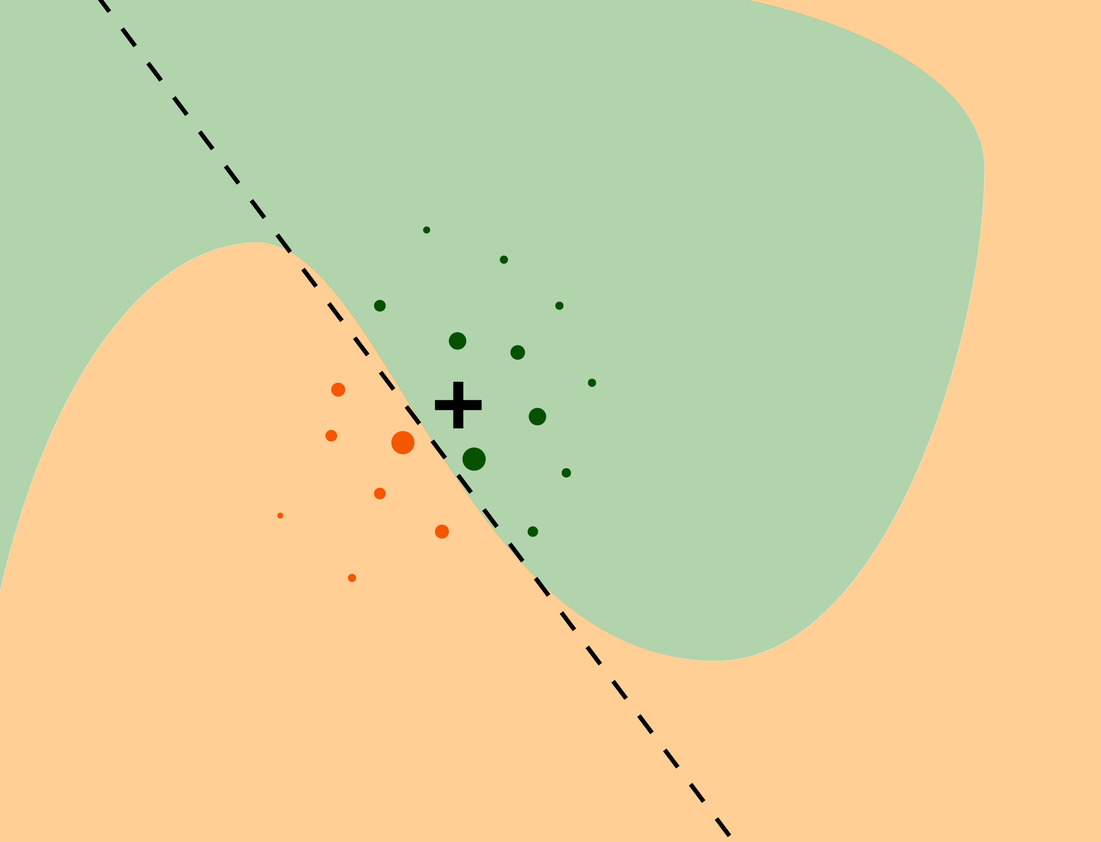
\(10\) nearest neighbors

Code

# prepare the recipe
prepped_rec_kknn <- extract_recipe(kknn_wf)

# write a function to bake the observation
bake_kknn <- function(x) {
  bake(
    prepped_rec_kknn,
    new_data = x
  )
}

# create explainer object
lime_explainer_kknn <- lime(
  x = scorecard_train,
  model = extract_fit_parsnip(kknn_wf),
  preprocess = bake_kknn
)

# top 5 features
explanation_kknn <- explain(
  x = both,
  explainer = lime_explainer_kknn,
  n_features = 10
)

plot_features(explanation_kknn) +
  theme_minimal(base_size = 12) +
  theme(legend.position = "bottom")

Random forest

Code

# prepare the recipe
prepped_rec_rf <- extract_recipe(rf_wf)

# write a function to bake the observation
bake_rf <- function(x) {
  bake(
    prepped_rec_rf,
    new_data = x
  )
}

# create explainer object
lime_explainer_rf <- lime(
  x = scorecard_train,
  model = extract_fit_parsnip(rf_wf),
  preprocess = bake_rf
)

# top 5 features
explanation_rf <- explain(
  x = both,
  explainer = lime_explainer_rf,
  n_features = 10
)

plot_features(explanation_rf) +
  theme_minimal(base_size = 12) +
  theme(legend.position = "bottom")

Additional resources

Underlying methods

Implementations in R

DALEX and DALEXtra
iml
lime
vip