Rows: 1
Columns: 12
$ state     <chr> "NY"
$ type      <fct> "Private, nonprofit"
$ admrate   <dbl> 0.0869
$ satavg    <dbl> 1510
$ cost      <dbl> 77047
$ netcost   <dbl> 29011
$ avgfacsal <dbl> 141849
$ pctpell   <dbl> 0.1737
$ comprate  <dbl> 0.9414
$ firstgen  <dbl> 0.154164
$ debt      <dbl> 13000
$ locale <fct> CityExplaining machine learning models
Lecture 24
Dr. Benjamin Soltoff
Cornell University
INFO 3312/5312 - Spring 2025
April 25, 2024
Announcements
Announcements
- Project 02 peer review
Goals
TODO
Review: Explanation
Explanation
Answer to the “why” question
Good explanations are
- Contrastive: why was this prediction made instead of another prediction?
- Selected: Focuses on just a handful of reasons, even if the problem is more complex
- Social: Needs to be understandable by your audience
- Truthful: Explanation should predict the event as truthfully as possible
- Generalizable: Explanation could apply to many predictions
- Explanation \(\leadsto\) local methods
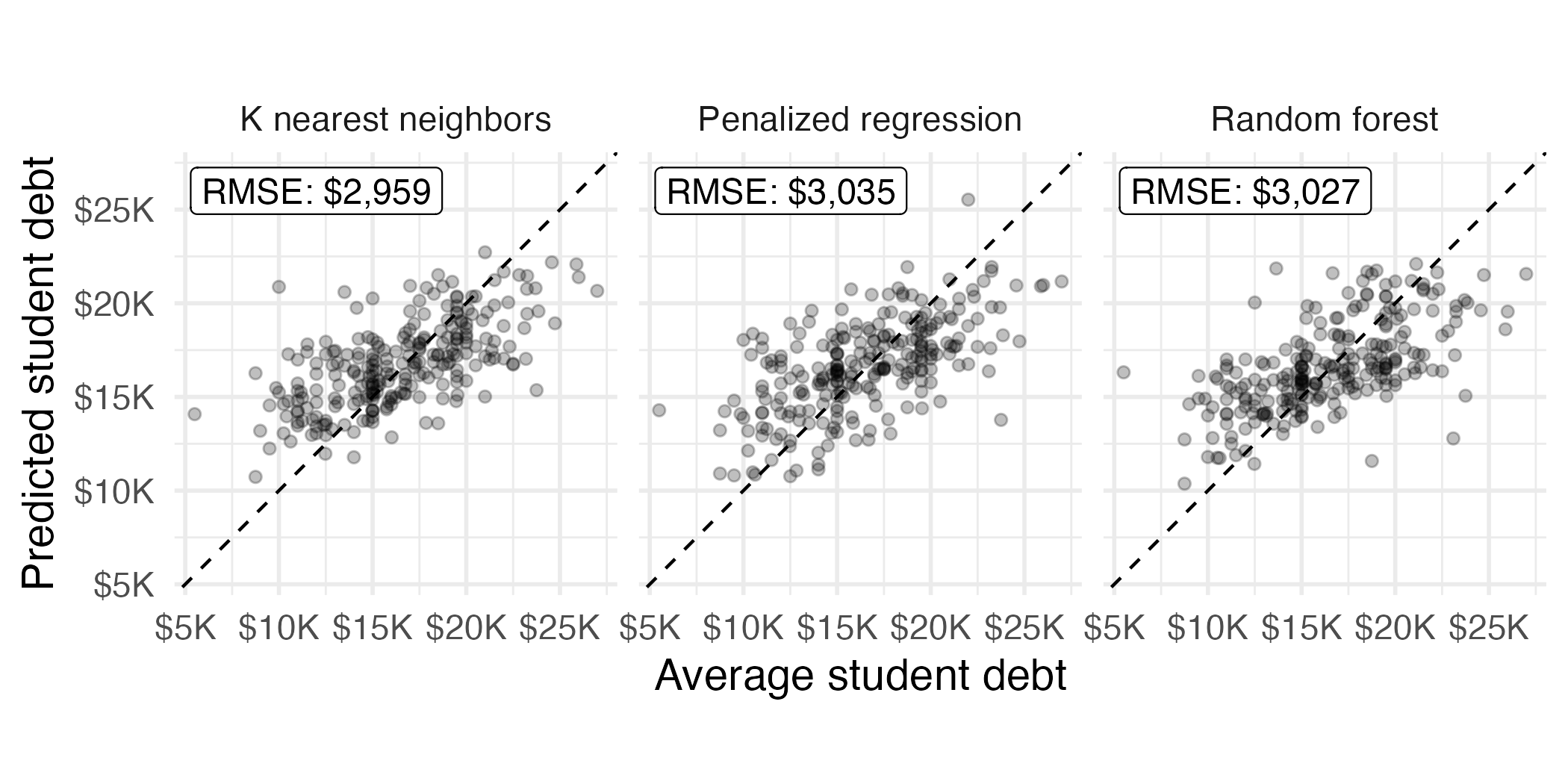
Evaluating test set performance
Local explanations
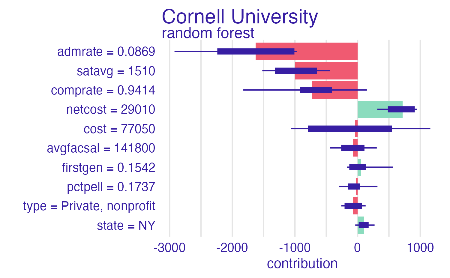
Cornell University
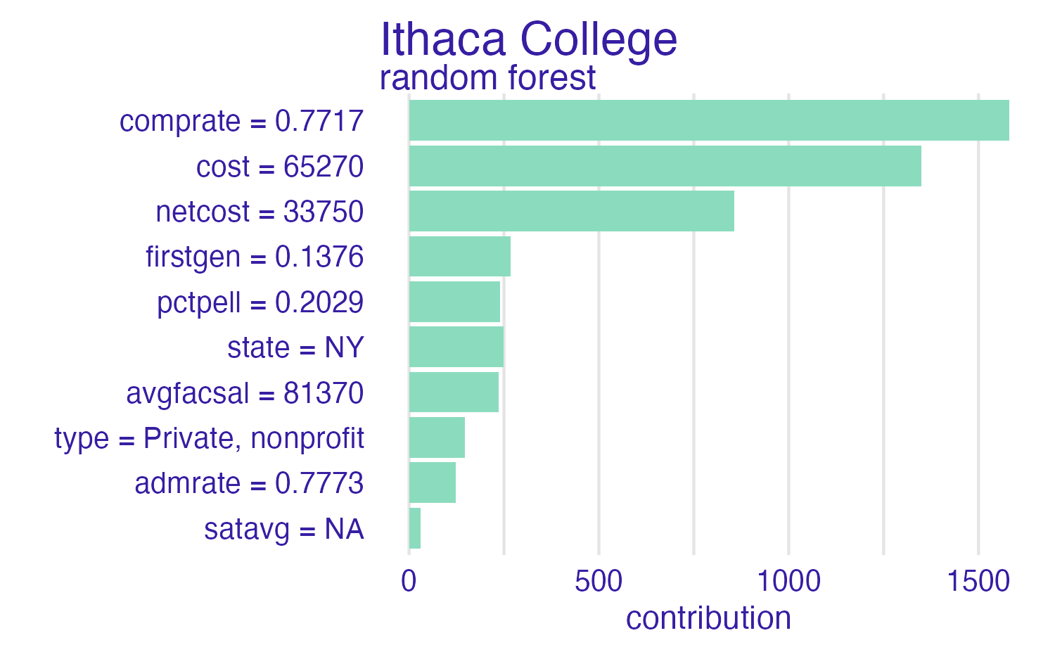
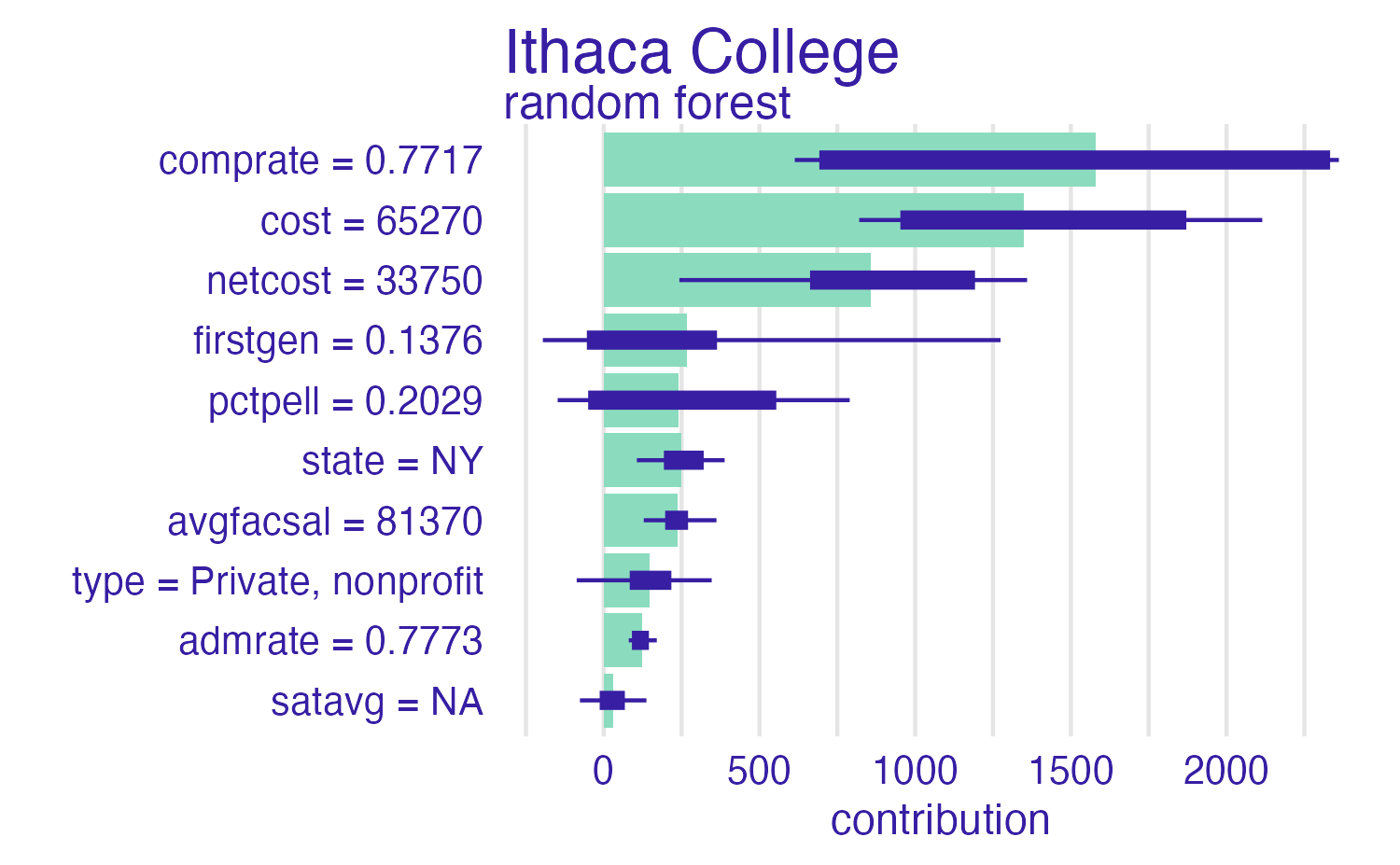
Ithaca College
Rows: 1
Columns: 12
$ state     <chr> "NY"
$ type      <fct> "Private, nonprofit"
$ admrate   <dbl> 0.7773
$ satavg    <dbl> NA
$ cost      <dbl> 65274
$ netcost   <dbl> 33748
$ avgfacsal <dbl> 81369
$ pctpell   <dbl> 0.2029
$ comprate  <dbl> 0.7717
$ firstgen  <dbl> 0.1375752
$ debt      <dbl> 19500
$ locale    <fct> Suburb
Break it down

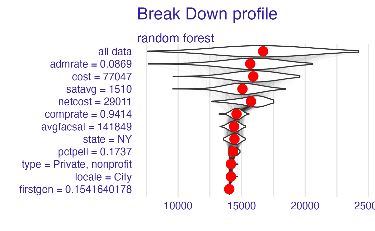
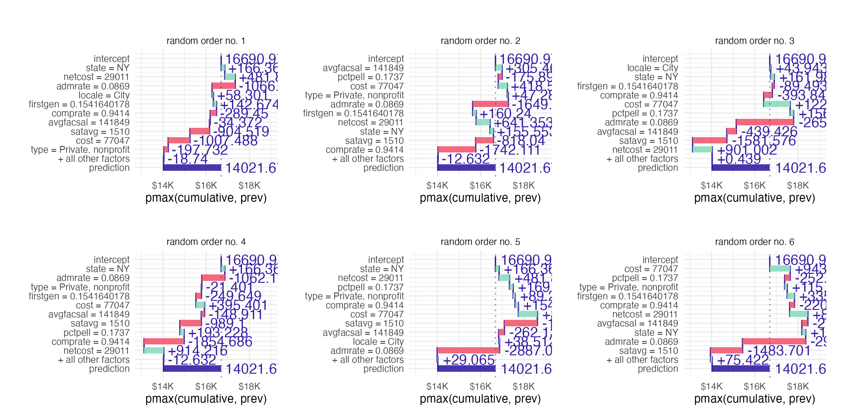
Breakdown methods
- How contributions attributed to individual features change the mean model’s prediction for a particular observation
- Sequentially fix the value of individual features and examine the change in the prediction
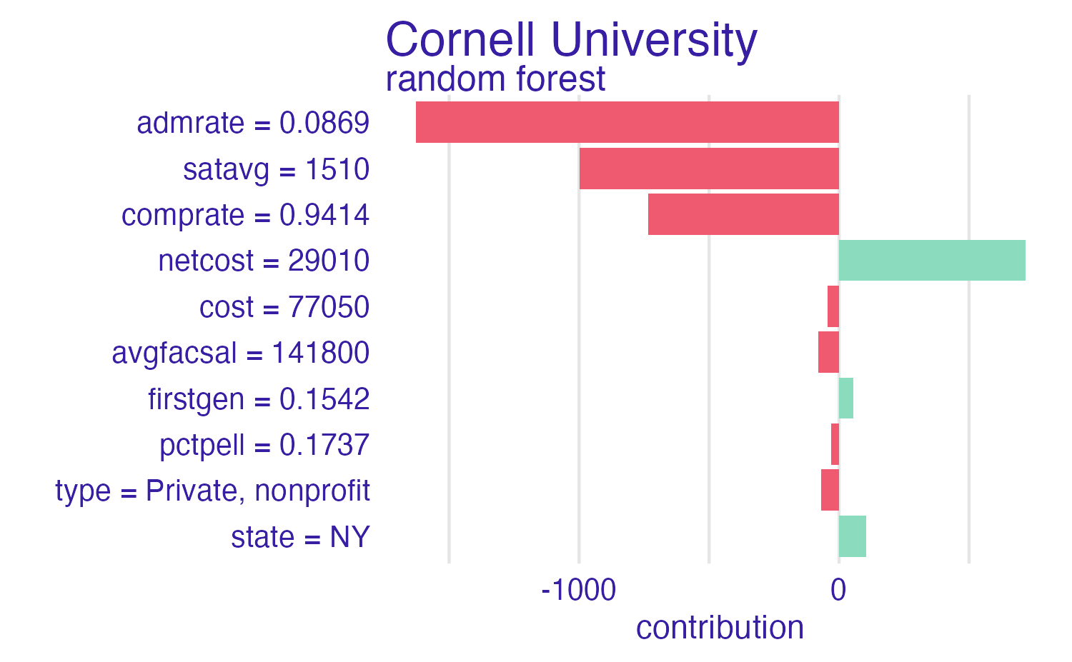
Breakdown of Cornell University using the random forest model

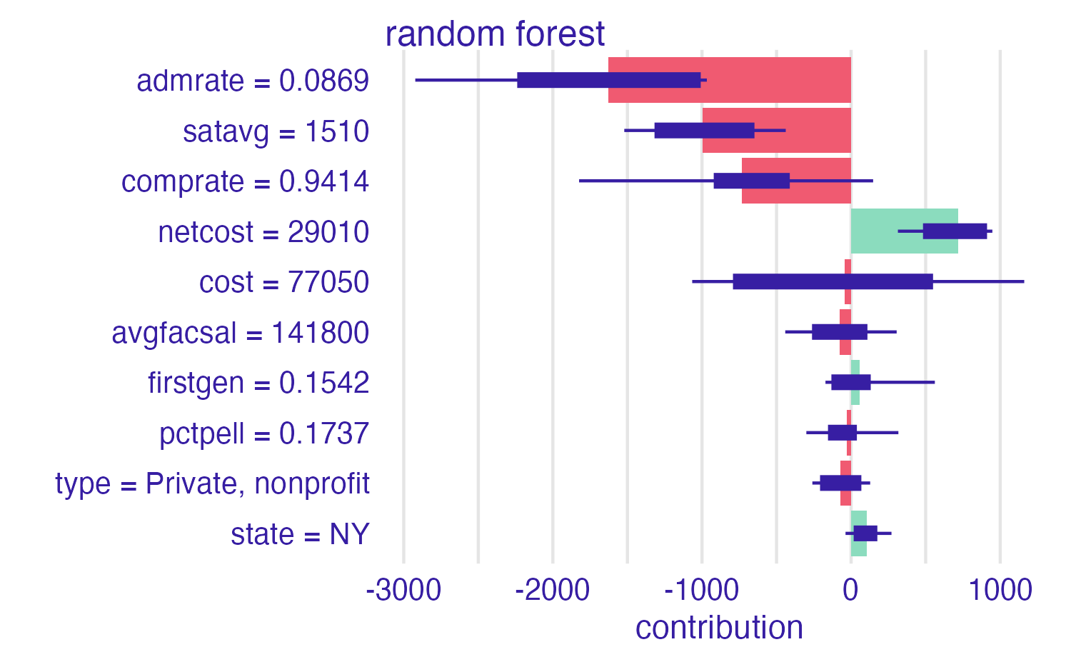
Break it down again
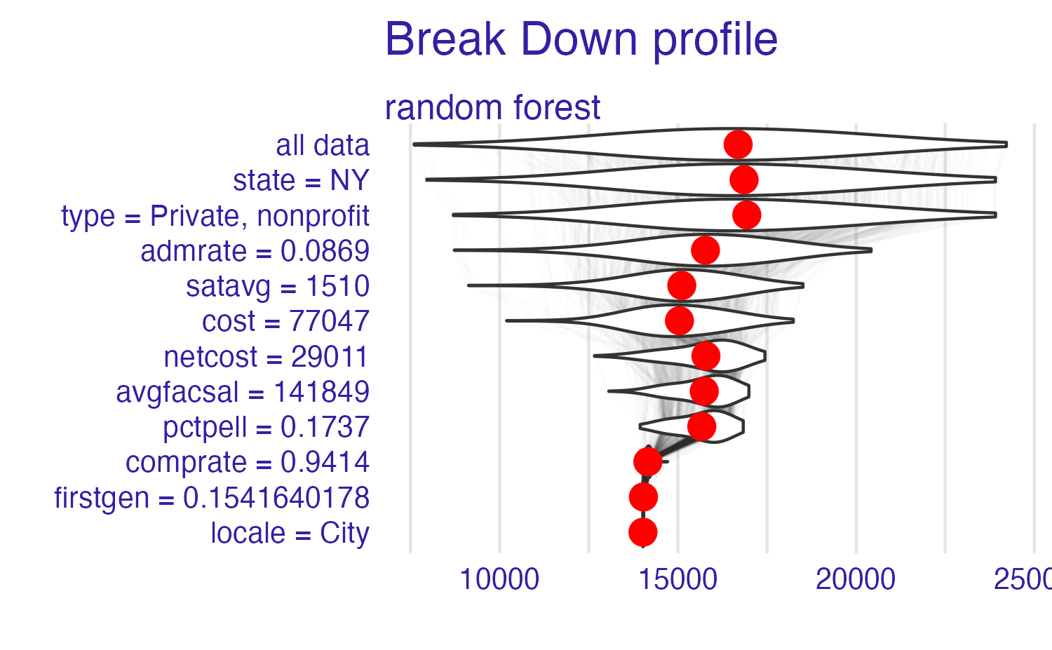
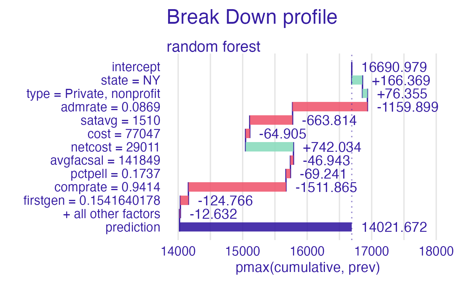
Breakdown of random forest
Breakdown plots
Advantages
- Easy to understand
- Compact visualization
- Intuitive explanation for linear models
Disadvantages
- Ignores interactive contributions (assumes everything is additive)
- Ordering of the explanatory variables influences the breakdown and resulting explanation
- Harder to interpret for models with lost of predictors
Shapley Additive Explanations (SHAP)
Shapley Additive Explanations (SHAP)
- Average contributions of features are computed under different coalitions of feature orderings
- Randomly permute feature order using \(B\) combinations
- Average across individual breakdowns to calculate feature contribution to individual prediction
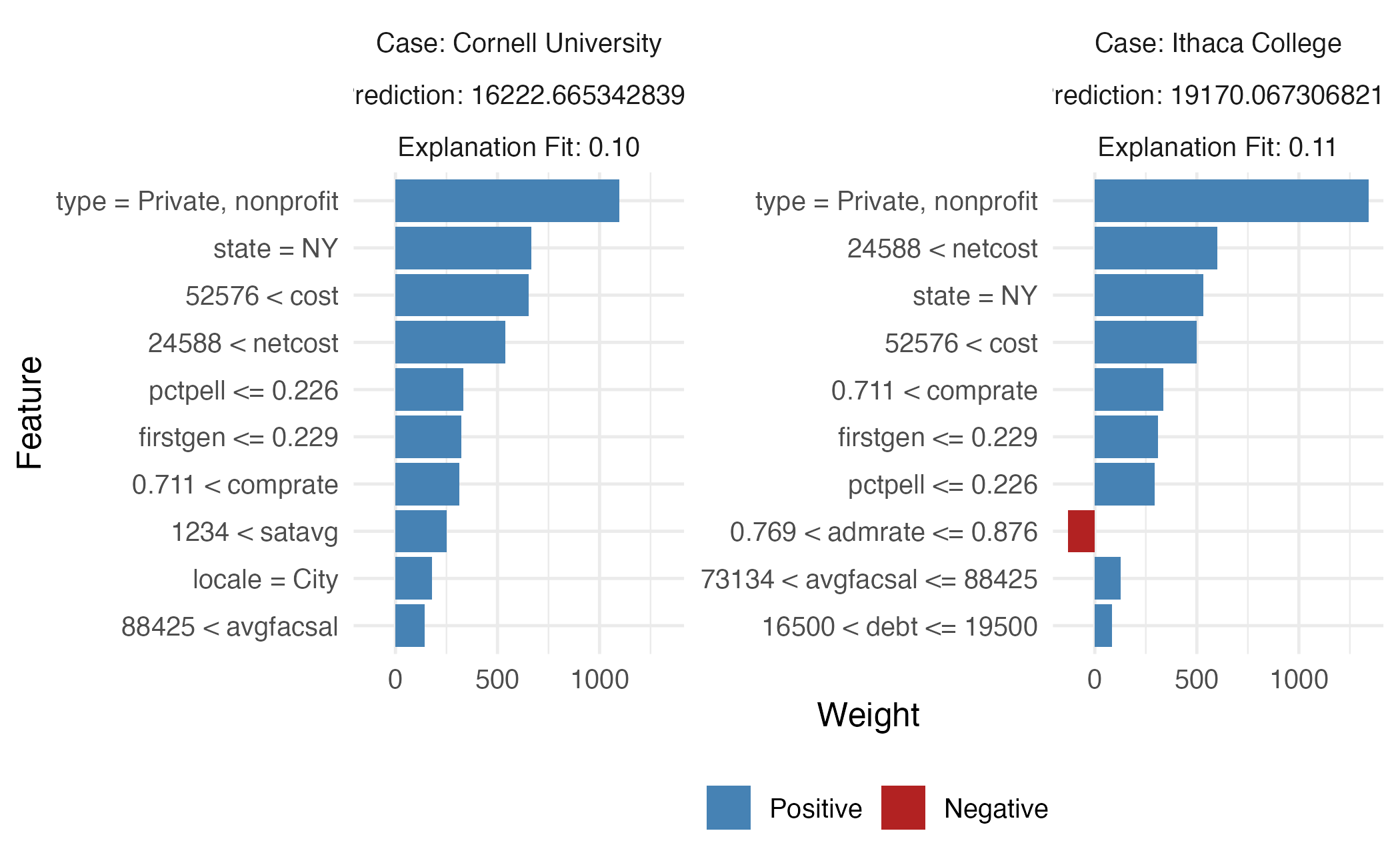
SHAP for Cornell
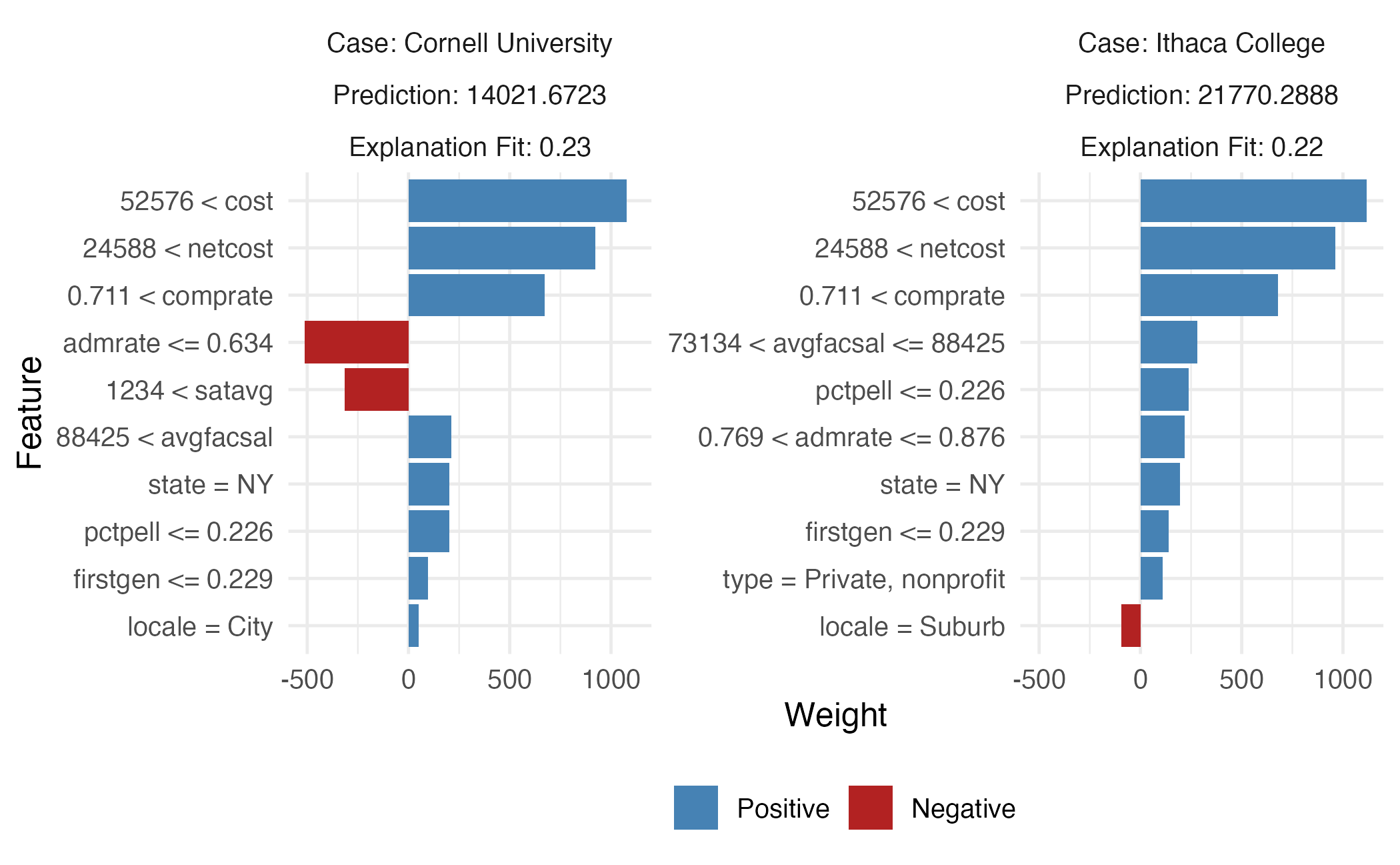
Cornell University vs. Ithaca College
Cornell University vs. Ithaca College
Shapley values
Advantages
- Model-agnostic
- Strong formal foundation from game theory
- Considers all (or many) possible feature orderings
Disadvantages
- Ignores interactive contributions (assumes everything is additive)
- Larger number of predictors makes it impossible to consider all possible coalitions
- Computationally expensive
Local interpretable model-agnostic explanations (LIME)
LIME
Local interpretable model-agnostic explanations
- Global \(\rightarrow\) local
- Interpretable model used to explain individual predictions of a black box model
- Assumes every complex model is linear on a local scale
- Simple model explains the predictions of the complex model locally
- Local fidelity
- Does not require global fidelity
- Works on tabular, text, and image data
LIME
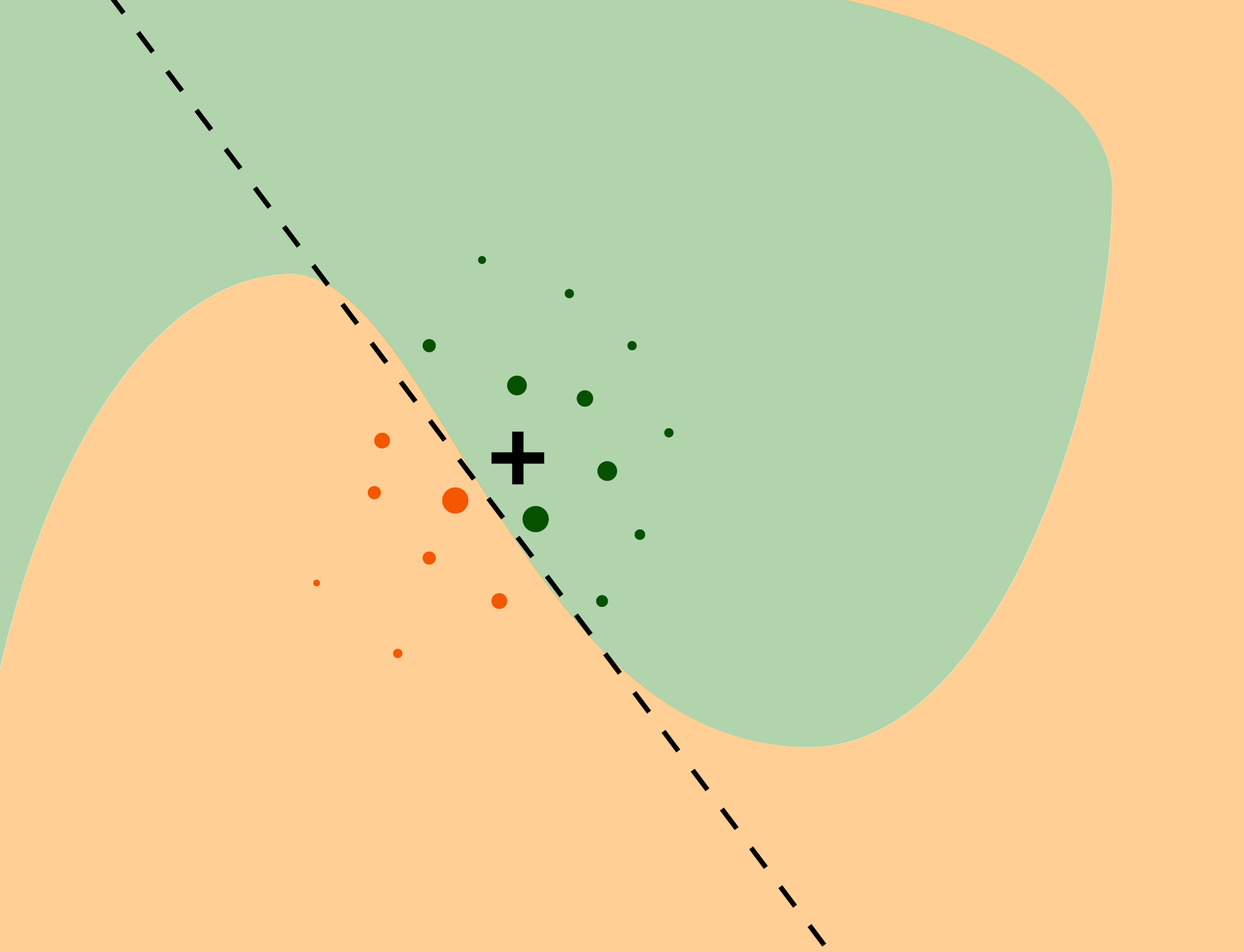
Source: Explanatory Model Analysis
LIME procedure
- For each prediction to explain, permute the observation \(n\) times
- Let the complex model predict the outcome of all permuted observations
- Calculate the distance from all permutations to the original observation
- Convert the distance to a similarity score
- Select \(m\) features best describing the complex model outcome from the permuted data
- Fit a simple model to the permuted data, explaining the complex model outcome with the \(m\) features from the permuted data weighted by its similarity to the original observation
- Extract the feature weights from the simple model and use these as explanations for the complex models local behavior
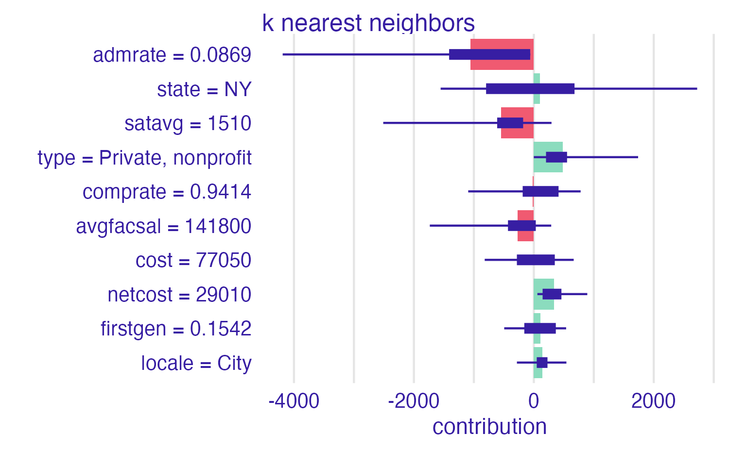
\(10\) nearest neighbors
Random forest
Binning continuous variables
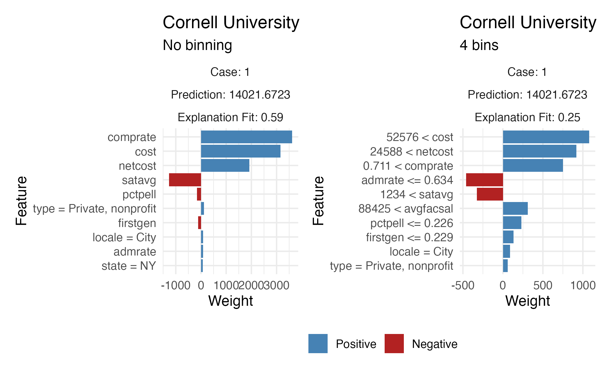
LIME
Advantages
- Can choose different local surrogates (e.g. regression model, decision tree)
- Local surrogates have their own set of interpretable features
- Explanations tend to be short and (maybe) contrastive
- Works for tabular data, text, and images
Disadvantages
- Hard to define the local “neighborhood”
- Explanations tend to be unstable
Application exercise
ae-21
- Go to the course GitHub org and find your
ae-21(repo name will be suffixed with your GitHub name). - Clone the repo in RStudio Workbench, open the Quarto document in the repo, and follow along and complete the exercises.
Wrap-up
Wrap-up
TODO
Additional resources
- Interpretable Machine Learning: A Guide for Making Black Box Models Explainable by Christoph Molnar
- Explanatory Model Analysis by Przemyslaw Biecek and Tomasz Burzykowski