Interactive reporting with Shiny (II)

Lecture 23

Dr. Benjamin Soltoff

Cornell University
INFO 3312/5312 - Spring 2026

April 21, 2026

Announcements

Project 02 draft

Learning objectives

Implement complex reactive features in Shiny
Implement dynamic UIs

Application exercise

`ae-22`

Instructions

Go to the course GitHub org and find your ae-22 (repo name will be suffixed with your GitHub name).
Clone the repo in Positron, run renv::restore() to install the required packages, open the Quarto document in the repo, and follow along and complete the exercises.
Render, commit, and push your edits by the AE deadline – end of the day

Where we left off last time

Reactive graph (again)

`reactive()`

DRY (Don’t Repeat Yourself)

Some of you may have noticed that in ex-03-A.R we have a bit of repeated code - specifically the filtering of d to subset the data for the selected airport.

While this is not a big deal here, it can become problematic in more complex apps.

exercises/ex-03-A.R

library(tidyverse)
library(shiny)
library(bslib)

d <- read_csv(here::here("data/weather.csv"))

d_vars <- c(
  "Average temp" = "temp_avg",
  "Min temp" = "temp_min",
  "Max temp" = "temp_max",
  "Total precip" = "precip",
  "Snow depth" = "snow",
  "Wind direction" = "wind_direction",
  "Wind speed" = "wind_speed",
  "Air pressure" = "air_press"
)

ui <- page_sidebar(
  title = "Weather Forecasts",
  sidebar = sidebar(
    radioButtons(
      "name",
      "Select an airport",
      choices = c(
        "Raleigh-Durham",
        "Houston Intercontinental",
        "Denver",
        "Los Angeles",
        "John F. Kennedy"
      )
    ),
    selectInput(
      "var",
      "Select a variable",
      choices = d_vars,
      selected = "temp_avg"
    )
  ),
  plotOutput("plot"),
  tableOutput("minmax")
)

server <- function(input, output, session) {
  output$plot <- renderPlot({
    d |>
      filter(name %in% input$name) |>
      ggplot(mapping = aes(x = date, y = .data[[input$var]])) +
      geom_line() +
      labs(title = str_c(input$name, "-", input$var))
  })

  output$minmax <- renderTable({
    d |>
      filter(name %in% input$name) |>
      mutate(
        year = year(date) |> as.integer()
      ) |>
      summarize(
        `min avg temp` = min(temp_min),
        `max avg temp` = max(temp_max),
        .by = year
      )
  })
}

shinyApp(ui = ui, server = server)

Demo 03 - Enter `reactive()`

demos/demo-03.R

library(tidyverse)
library(shiny)
library(bslib)

d <- read_csv(here::here("data/weather.csv"))

d_vars <- c(
  "Average temp" = "temp_avg",
  "Min temp" = "temp_min",
  "Max temp" = "temp_max",
  "Total precip" = "precip",
  "Snow depth" = "snow",
  "Wind direction" = "wind_direction",
  "Wind speed" = "wind_speed",
  "Air pressure" = "air_press"
)

ui <- page_sidebar(
  title = "Weather Forecasts",
  sidebar = sidebar(
    radioButtons(
      "name",
      "Select an airport",
      choices = c(
        "Raleigh-Durham",
        "Houston Intercontinental",
        "Denver",
        "Los Angeles",
        "John F. Kennedy"
      )
    ),
    selectInput(
      "var",
      "Select a variable",
      choices = d_vars,
      selected = "temp_avg"
    )
  ),
  plotOutput("plot"),
  tableOutput("minmax")
)

server <- function(input, output, session) {
  d_city <- reactive({
    d |>
      filter(name %in% input$name)
  })

  output$plot <- renderPlot({
    d_city() |>
      ggplot(mapping = aes(x = date, y = .data[[input$var]])) +
      geom_line() +
      labs(title = str_c(input$name, "-", input$var))
  })

  output$minmax <- renderTable({
    d_city() |>
      mutate(
        year = year(date) |> as.integer()
      ) |>
      summarize(
        `min avg temp` = min(temp_min),
        `max avg temp` = max(temp_max),
        .by = year
      )
  })
}

shinyApp(ui = ui, server = server)

Another reactive expression

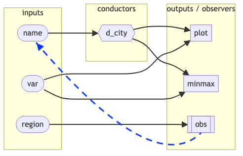
This is an example of a reactive conductor - it is a new type of reactive expression that exists between sources (e.g. an input) and endpoints (e.g. an output).

As such, a reactive() depends on various upstream inputs, returns a value of some kind which is used by 1 or more downstream outputs (or other conductors).

Their primary use is similar to a function in an R script, they help to

Avoid repeating ourselves
Decompose complex computations into smaller / more modular steps
Improve computational efficiency by breaking up / simplifying reactive dependencies

`reactive()` tips

Expressions are written in the same way as render*() functions but they do not have the output$ prefix.
```
react_obj <- reactive({
  ...
})
```

Any consumer of react_obj must access its value using react_obj() and not react_obj
- Think of react_obj as a function that returns the current value
- Common cause of the R error
```
## Error: object of type 'closure' is not subsettable`
```

Like input reactive expressions, may only be used within reactive contexts

## Error: Operation not allowed without an active reactive context. (You tried to do something that can only be done from inside a reactive expression or observer.)

Reactive graph

Observers

`observe()`

These are the final reactive expression we will be discussing. They are constructed in the same way as a reactive() however an observer does not return a value, instead they are used for their side effects.

Side effects in most cases involve sending data to the client browser, e.g. updating a UI element
While not obvious given their syntax - the results of the render*() functions are observers.

Demo 04 - filtering by region

demos/demo-04.R

library(tidyverse)
library(shiny)
library(bslib)

d <- read_csv(here::here("data/weather.csv"))

d_vars <- c(
  "Average temp" = "temp_avg",
  "Min temp" = "temp_min",
  "Max temp" = "temp_max",
  "Total precip" = "precip",
  "Snow depth" = "snow",
  "Wind direction" = "wind_direction",
  "Wind speed" = "wind_speed",
  "Air pressure" = "air_press"
)

ui <- page_sidebar(
  title = "Weather Forecasts",
  sidebar = sidebar(
    selectInput(
      "region",
      label = "Select a region",
      choices = c("West", "Midwest", "Northeast", "South")
    ),
    selectInput(
      "name",
      label = "Select an airport",
      choices = c()
    ),
    selectInput(
      "var",
      label = "Select a variable",
      choices = d_vars,
      selected = "temp_avg"
    )
  ),
  plotOutput("plot"),
  tableOutput("minmax")
)

server <- function(input, output, session) {
  observe({
    updateSelectInput(
      session = session,
      inputId = "name",
      choices = d |>
        distinct(region, name) |>
        filter(region == input$region) |>
        pull(name)
    )
  })

  d_city <- reactive({
    d |>
      filter(name %in% input$name)
  })

  output$plot <- renderPlot({
    d_city() |>
      ggplot(mapping = aes(x = date, y = .data[[input$var]])) +
      geom_line() +
      labs(title = str_c(input$name, "-", input$var))
  })

  output$minmax <- renderTable({
    d_city() |>
      mutate(
        year = year(date) |> as.integer()
      ) |>
      summarize(
        `min avg temp` = min(temp_min),
        `max avg temp` = max(temp_max),
        .by = year
      )
  })
}

shinyApp(ui = ui, server = server)

Reactive graph

Reactive graph - implicit

Using `req()`

You may have noticed that the App initializes with “West” selected for region but no initial selection for name. Because of this we have some warnings generated in the console:

# Warning: There were 2 warnings in `summarize()`.
# The first warning was:
# ℹ In argument: `min temp = min(temp_min)`.
# Caused by warning in `min()`:
# ! no non-missing arguments to min; returning Inf
# ℹ Run dplyr::last_dplyr_warnings() to see the 1 remaining warning.

This is a common occurrence with Shiny, particularly at initialization or when a user enters partial / bad input(s).

A good way to protect against this is to validate inputs before using them - the simplest way is to use req() which checks if a value is truthy and prevent further execution if not.

Truthiness in Shiny

In Shiny, “truthiness” determines whether a value should be considered valid for reactive execution.

A value is considered truthy if it is:

Not NULL
Not FALSE
Not an empty vector (character(0), numeric(0), etc.)
Not an empty string ""
Not NA

isTruthy(TRUE)

[1] TRUE

isTruthy(1)

[1] TRUE

isTruthy("hello")

[1] TRUE

isTruthy(c(1, 2, 3))

[1] TRUE

isTruthy(NULL)

[1] FALSE

isTruthy(FALSE)

[1] FALSE

isTruthy("")

[1] FALSE

isTruthy(character(0))

[1] FALSE

isTruthy(NA)

[1] FALSE

⌨️ Your turn - exercise 04

Instructions

Using the code provided in exercises/ex-04.R (based on demos/demo-04.R) as a starting point, add the calls to req() necessary to avoid the initialization warnings.

Also, think about if there are any other locations in our app where req() might be useful.

Tip

Thinking about how events “flow” through the reactive graph will be helpful here.

10:00

`req()` vs `validate()`

`req()`

Silently stop execution of a reactive expression if a condition is not met

d_city <- reactive({
  req(input$name)

  d |>
    filter(name %in% input$name)
})

`validate()`

Stop execution of a reactive expression and display an error message to the user if a condition is not met

d_city <- reactive({
  validate(
    need(input$name, "Please select an airport")
  )

  d |>
    filter(name %in% input$name)
})

A note on observers

Reactive graphs are meant to be acyclic, that is they should not have circular dependencies.

The use of observers can introduce cycles (accidentally) which can then lead to infinite loops, see the following example:

library(shiny)

ui = fluidPage(
  numericInput("n", "n", 0)
)

server = function(input, output, session) {
  observe({
    updateNumericInput(inputId = "n", value = input$n + 1)
  }) |>
    bindEvent(input$n)
}

shinyApp(ui = ui, server = server)

Downloading from Shiny

`downloadButton()`

is a special UI input widget designed to launch a download window from your Shiny app.

downloadButton() is a special case of an actionButton() with specialized server syntax. These are different from the other inputs we’ve used so far, as they are primarily used to trigger an action rather than return a value.

Rather than using an observe() or render*(), this widget is paired with the special downloadHandler() function which uses the latter’s syntax in our server function.

`downloadHandler()`

Specifically, within our server definition we attach the downloadHandler() to the downloadButton’s id via output, e.g.

output$download_btn = downloadHandler(...)

The handler then defines two functions:

filename(), which is a function that generates a default filename
content(), which is a function that writes the file’s content to a temporary location

Demo 05 - A download button

demos/demo-05.R

library(tidyverse)
library(shiny)
library(bslib)

d <- read_csv(here::here("data/weather.csv"))

d_vars <- c(
  "Average temp" = "temp_avg",
  "Min temp" = "temp_min",
  "Max temp" = "temp_max",
  "Total precip" = "precip",
  "Snow depth" = "snow",
  "Wind direction" = "wind_direction",
  "Wind speed" = "wind_speed",
  "Air pressure" = "air_press"
)

ui <- page_sidebar(
  title = "Weather Forecasts",
  sidebar = sidebar(
    selectInput(
      "region",
      "Select a region",
      choices = sort(unique(d$region)),
      selected = "West"
    ),
    selectInput(
      "name",
      "Select an airport",
      choices = c()
    ),
    selectInput(
      "var",
      "Select a variable",
      choices = d_vars,
      selected = "temp_avg"
    ),
    downloadButton("download")
  ),
  plotOutput("plot")
)

server <- function(input, output, session) {
  output$download <- downloadHandler(
    filename = function() {
      name = input$name |>
        str_replace_all(" ", "_") |>
        str_to_lower()
      str_c(name, ".csv", collapse = "")
    },
    content = function(file) {
      write_csv(d_city(), file)
    }
  )

  d_city <- reactive({
    req(input$name)
    d |>
      filter(name %in% input$name)
  })

  observe({
    updateSelectInput(
      session,
      "name",
      choices = d |>
        distinct(region, name) |>
        filter(region == input$region) |>
        pull(name)
    )
  })

  output$plot <- renderPlot({
    d_city() |>
      ggplot(mapping = aes(x = date, y = .data[[input$var]])) +
      ggtitle(input$var) +
      geom_line() +
      theme_minimal()
  })
}

shinyApp(ui = ui, server = server)

Controlling the reactive graph

For both observers, reactives, and render functions, Shiny will automatically determine reactive dependencies for you - in some cases this is not what we want.

To explicitly control the dependencies of these reactive expressions we can modify them using bindEvent() to define the dependencies explicitly.

The first argument is the reactive expression to modify and the following is the inputs and reactives that should trigger it.

Demo 06 - A fancier download experience

demos/demo-06.R

library(tidyverse)
library(shiny)
library(bslib)

d <- read_csv(here::here("data/weather.csv"))

d_vars <- c(
  "Average temp" = "temp_avg",
  "Min temp" = "temp_min",
  "Max temp" = "temp_max",
  "Total precip" = "precip",
  "Snow depth" = "snow",
  "Wind direction" = "wind_direction",
  "Wind speed" = "wind_speed",
  "Air pressure" = "air_press"
)

ui <- page_sidebar(
  title = "Weather Forecasts",
  sidebar = sidebar(
    selectInput(
      "region",
      "Select a region",
      choices = sort(unique(d$region)),
      selected = "West"
    ),
    selectInput(
      "name",
      "Select an airport",
      choices = c()
    ),
    selectInput(
      "var",
      "Select a variable",
      choices = d_vars,
      selected = "temp"
    ),
    actionButton("export_modal", "Export data")
  ),
  plotOutput("plot")
)

server <- function(input, output, session) {
  observe({
    showModal(
      modalDialog(
        title = "Download data",
        dateRangeInput(
          "dl_dates",
          "Select date range",
          start = min(d_city()$date),
          end = max(d_city()$date)
        ),
        checkboxGroupInput(
          "dl_vars",
          "Select variables to download",
          choices = names(d),
          selected = names(d),
          inline = TRUE
        ),
        footer = list(
          downloadButton("download"),
          modalButton("Cancel")
        )
      )
    )
  }) |>
    bindEvent(input$export_modal)

  output$download <- downloadHandler(
    filename = function() {
      name = input$name |>
        str_replace_all(" ", "_") |>
        str_to_lower()
      str_c(name, ".csv", collapse = "")
    },
    content = function(file) {
      write_csv(
        d_city() |>
          filter(date >= input$dl_dates[1] & date <= input$dl_dates[2]) |>
          select(input$dl_vars),
        file
      )
    }
  )

  d_city <- reactive({
    req(input$name)
    d |>
      filter(name %in% input$name)
  })

  observe({
    updateSelectInput(
      inputId = "name",
      choices = d |>
        filter(region == input$region) |>
        pull(name) |>
        unique() |>
        sort()
    )
  })

  output$plot <- renderPlot({
    d_city() |>
      ggplot(mapping = aes(x = date, y = .data[[input$var]])) +
      ggtitle(input$var) +
      geom_line() +
      theme_minimal()
  })
}

shinyApp(ui = ui, server = server)

Uploading to Shiny

`fileInput()` widget

This widget behaves a bit differently than the others we have seen - like the other widgets it returns a value via input$<id> but the value returned changes based on whether or not a file has been uploaded.

Specifically, before the file is uploaded, the input will return NULL. After file(s) are uploaded the input returns a data frame with one row per file and the following columns:

name - the original filename (from the client’s system)
size - file size in bytes
type - file mime type, usually determined by the file extension
datapath - location of the temporary file on the server

Your app is then responsible for reading in and processing the uploaded file(s) as needed.

Using `fileInput()`

library(tidyverse)
library(shiny)
library(bslib)

ui = page_fluid(
  fileInput("upload", "Upload a file", accept = ".csv"),
  h3("Result:"),
  tableOutput("result"),
  h3("Content:"),
  tableOutput("data")
)

server = function(input, output, session) {
  output$result = renderTable({
    req(input$upload)
    input$upload
  })
  
  output$data = renderTable({
    req(input$upload)
    ext = tools::file_ext(input$upload$datapath)
    
    validate(
      need(ext == "csv", "Please upload a csv file")
    )
    
    readr::read_csv(input$upload$datapath) |>
      head()
  })
}

shinyApp(ui = ui, server = server)

`fileInput()` hints

input$upload will default to NULL when the app is loaded, using req(input$upload) for downstream consumers prevents errors/warnings until a file is uploaded
Files in datapath are temporary and should be treated as ephemeral, additional uploads can result in previous files being deleted
type is at best a guess - validate uploaded files and write defensive code
The accept argument helps to limit file types but cannot prevent bad uploads

⌨️ Your turn - exercise 05

Instructions

Starting with the code in exercises/ex-05.R replace the preloading of the weather data, d, with a reactive() version that is populated via a fileInput() widget.

You should then be able to get the same app behavior as before once data/weather.csv is uploaded. You can also check that your app works with the smaller data/jfk_weather.csv dataset as well.

Tip

Remember that anywhere that uses either d will now need to use d() instead.

12:00

Wrap-up

Recap

Explicitly define reactive dependencies using bindEvent()
Use modals for popup dialog that don’t permanently clutter the UI

Acknowledgements

Slides derived in part from posit::conf 2025 - Shiny for R Workshop by Colin Rundel and licensed under a Creative Commons Attribution 4.0 International License.

Interactive reporting with Shiny (II)

Announcements

Announcements

Learning objectives

Application exercise

ae-22

Where we left off last time

Reactive graph (again)

reactive()

DRY (Don’t Repeat Yourself)

Demo 03 - Enter reactive()

Another reactive expression

reactive() tips

Reactive graph

Observers

observe()

Demo 04 - filtering by region

Reactive graph

Reactive graph - implicit

Using req()

Truthiness in Shiny

⌨️ Your turn - exercise 04

req() vs validate()

req()

validate()

A note on observers

Downloading from Shiny

downloadButton()

downloadHandler()

Demo 05 - A download button

Controlling the reactive graph

Modal dialogs

Demo 06 - A fancier download experience

Uploading to Shiny

fileInput() widget

Using fileInput()

fileInput() hints

⌨️ Your turn - exercise 05

Wrap-up

Recap

Acknowledgements

`ae-22`

`reactive()`

Demo 03 - Enter `reactive()`

`reactive()` tips

`observe()`

Using `req()`

`req()` vs `validate()`

`req()`

`validate()`

`downloadButton()`

`downloadHandler()`

`fileInput()` widget

Using `fileInput()`

`fileInput()` hints