Rows: 1,719
Columns: 14
$ unitid    <dbl> 100654, 100663, 100706, 100724, 100751, 100830, 100858, 1009…
$ name      <chr> "Alabama A & M University", "University of Alabama at Birmin…
$ state     <chr> "AL", "AL", "AL", "AL", "AL", "AL", "AL", "AL", "AL", "AL", …
$ type      <fct> "Public", "Public", "Public", "Public", "Public", "Public", …
$ admrate   <dbl> 0.7160, 0.8854, 0.7367, 0.9799, 0.7890, 0.9680, 0.7118, 0.65…
$ satavg    <dbl> 954, 1266, 1300, 955, 1244, 1069, NA, 1214, 1042, NA, 1111, …
$ cost      <dbl> 21924, 26248, 24869, 21938, 31050, 20621, 32678, 33920, 3645…
$ netcost   <dbl> 13057, 16585, 17250, 13593, 21534, 13689, 23258, 21098, 2037…
$ avgfacsal <dbl> 79011, 104310, 88380, 69309, 94581, 70965, 99837, 68724, 564…
$ pctpell   <dbl> 0.6853, 0.3253, 0.2377, 0.7205, 0.1712, 0.4821, 0.1301, 0.21…
$ comprate  <dbl> 0.2807, 0.6245, 0.6072, 0.2843, 0.7223, 0.3569, 0.8088, 0.69…
$ firstgen  <dbl> 0.3658281, 0.3412237, 0.3101322, 0.3434343, 0.2257127, 0.381…
$ debt      <dbl> 16600, 15832, 13905, 17500, 17986, 13119, 17750, 16000, 1500…
$ locale <fct> City, City, City, City, City, City, City, City, City, Suburb…Interpreting machine learning models
Lecture 23
Dr. Benjamin Soltoff
Cornell University
INFO 3312/5312 - Spring 2025
April 23, 2024
Announcements
Announcements
- Homework 06
- Friday lab: peer review of draft projects
Goals
- Review the importance of interpretability for machine learning models
- Estimate permutation-based feature importance measures
- Evaluate marginal effects of features using partial dependence plots
- Generate global surrogates to interpret black-box models
Review: Interpretability
Interpretation
- How does this model work?
- Interpretation \(\leadsto\) global methods
- White-box models lend themselves naturally to interpretation
- Black-box models require additional effort
- Prefer model-agnostic methods
Packages for model interpretation
Packages for model interpretation
As of 2020,1 over 30 packages with functions for model interpretation are available in R. Some of the most popular ones include:
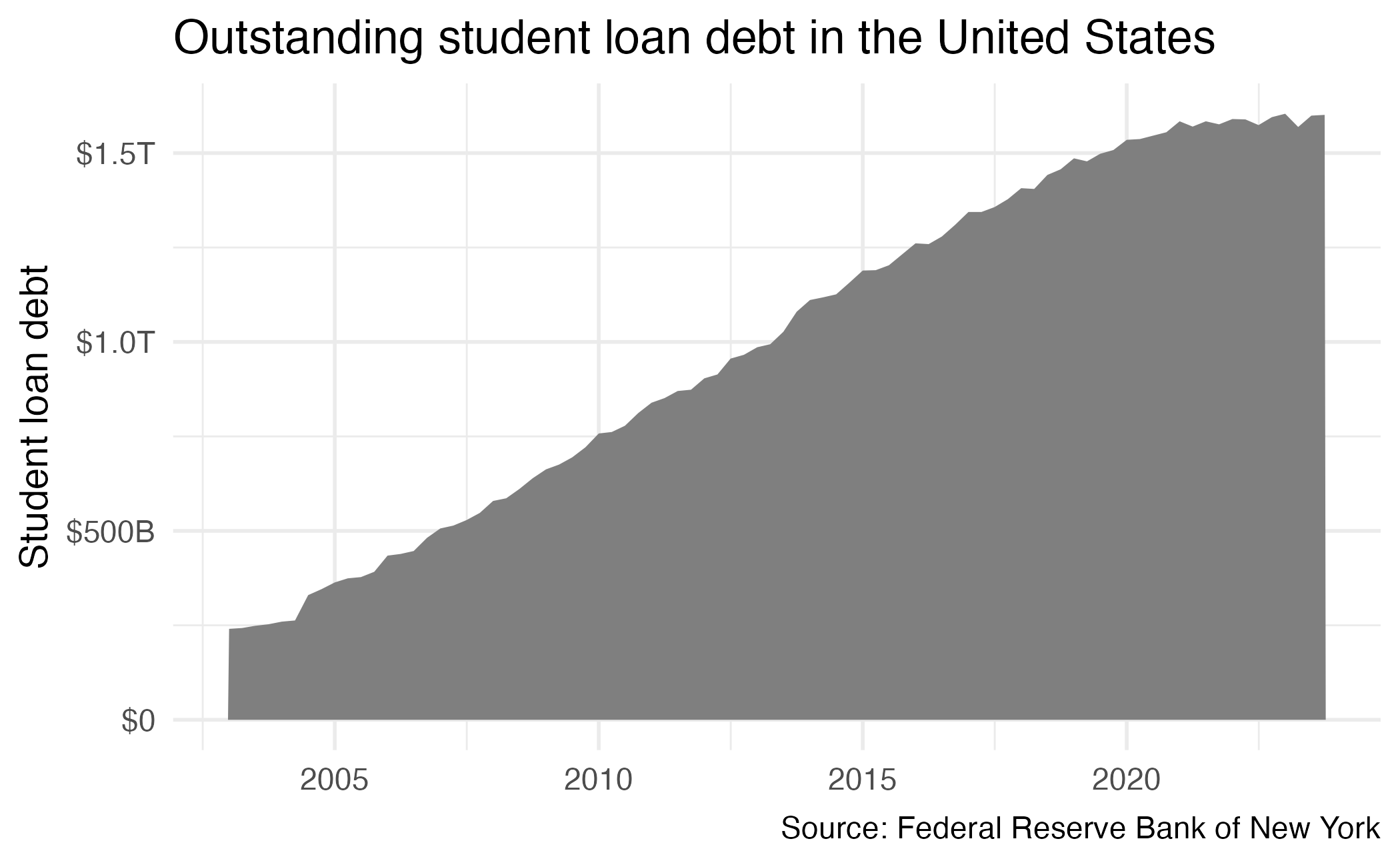
Predicting student debt
ae-20
- Go to the course GitHub org and find your
ae-20(repo name will be suffixed with your GitHub name). - Clone the repo in RStudio Workbench, open the Quarto document in the repo, and follow along and complete the exercises.
Predicting student debt
- College Scorecard
- rscorecard
rcis::scorecard
Predicting student debt
Fitted models
library(tidyverse)
library(tidymodels)
library(rcis)
library(here)
# get scorecard dataset
data("scorecard")
scorecard <- scorecard |>
# remove ID columns - causing issues when interpreting/explaining
select(-unitid, -name) |>
# convert factor to character columns
mutate(across(.cols = where(is.factor), .f = as.character))
# split into training and testing
set.seed(123)
scorecard_split <- initial_split(data = scorecard, prop = .75, strata = debt)
scorecard_train <- training(scorecard_split)
scorecard_test <- testing(scorecard_split)
scorecard_folds <- vfold_cv(data = scorecard_train, v = 10)
# basic feature engineering recipe
scorecard_rec <- recipe(debt ~ ., data = scorecard_train) |>
# catch all category for missing state values
step_novel(state) |>
# use median imputation for numeric predictors
step_impute_median(all_numeric_predictors()) |>
# use modal imputation for nominal predictors
step_impute_mode(all_nominal_predictors()) |>
# remove rows with missing values for
# outcomes - glmnet won't work if any of this column is NA
step_naomit(all_outcomes())
# generate random forest model
rf_mod <- rand_forest() |>
set_engine("ranger") |>
set_mode("regression")
# combine recipe with model
rf_wf <- workflow() |>
add_recipe(scorecard_rec) |>
add_model(rf_mod)
# fit using training set
set.seed(123)
rf_wf <- fit(
rf_wf,
data = scorecard_train
)
# fit penalized regression model
## recipe
glmnet_recipe <- scorecard_rec |>
# use median imputation for numeric predictors
step_impute_median(all_numeric_predictors()) |>
step_dummy(all_nominal_predictors()) |>
step_zv(all_predictors()) |>
step_normalize(all_numeric_predictors())
## model specification
glmnet_spec <- linear_reg(penalty = tune(), mixture = tune()) |>
set_mode("regression") |>
set_engine("glmnet")
## workflow
glmnet_workflow <- workflow() |>
add_recipe(glmnet_recipe) |>
add_model(glmnet_spec)
## tuning grid
glmnet_grid <- expand_grid(
penalty = 10^seq(-6, -1, length.out = 20),
mixture = c(0.05, 0.2, 0.4, 0.6, 0.8, 1)
)
## hyperparameter tuning
glmnet_tune <- tune_grid(
glmnet_workflow,
resamples = scorecard_folds,
grid = glmnet_grid
)
# select best model
glmnet_best <- select_best(glmnet_tune, metric = "rmse")
glmnet_wf <- finalize_workflow(glmnet_workflow, glmnet_best) |>
last_fit(scorecard_split) |>
extract_workflow()
# nearest neighbors model
## use glmnet recipe
kknn_spec <- nearest_neighbor(neighbors = 10) |>
set_mode("regression") |>
set_engine("kknn")
kknn_workflow <-
workflow() |>
add_recipe(glmnet_recipe) |>
add_model(kknn_spec)
## fit using training set
set.seed(123)
kknn_wf <- fit(
kknn_workflow,
data = scorecard_train
)
# save all required objects to a .Rdata file
save(scorecard_train, scorecard_test, rf_wf, glmnet_wf, kknn_wf,
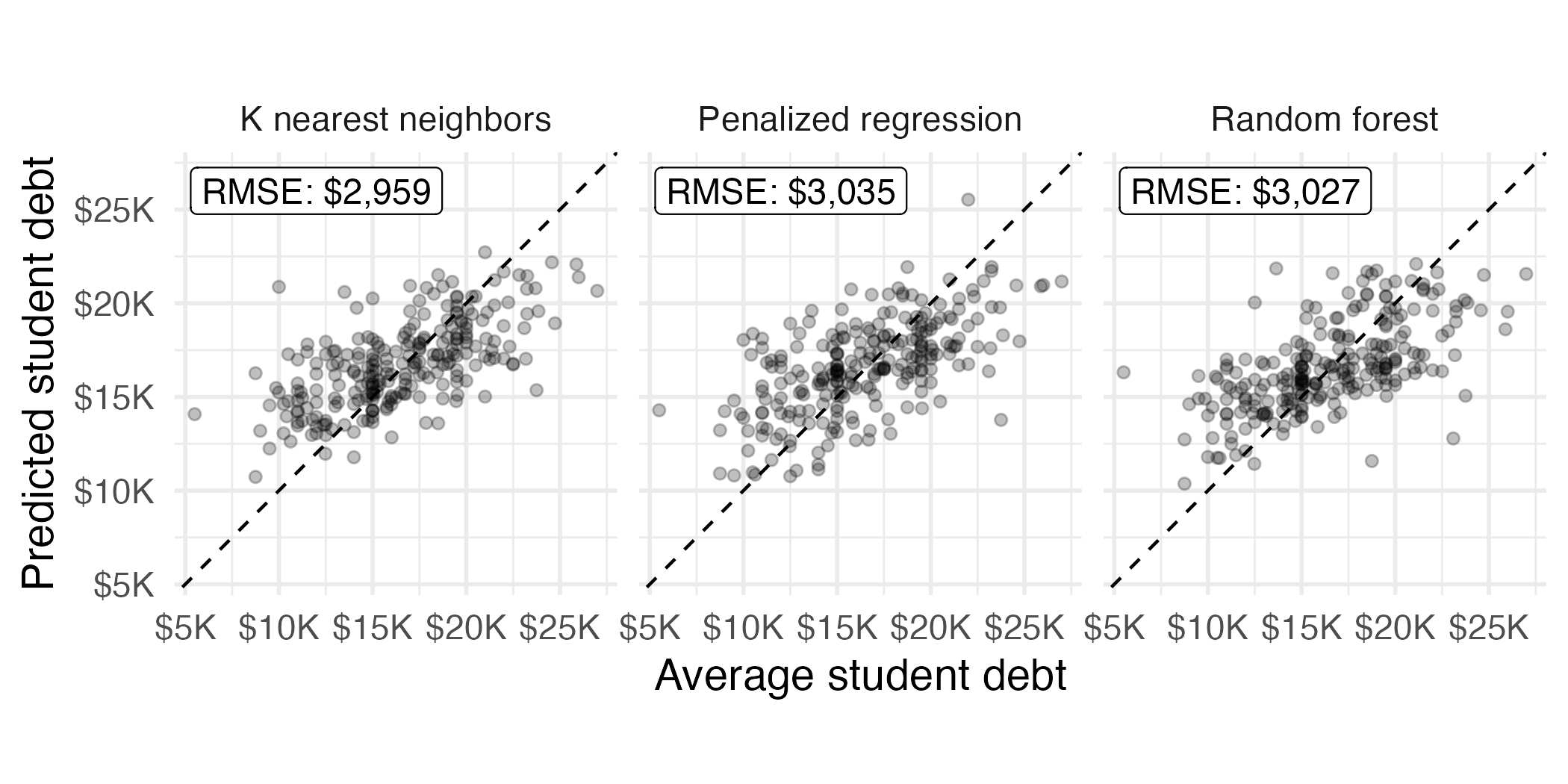
file = here("ae/data/scorecard-models.RData"))Evaluating test set performance
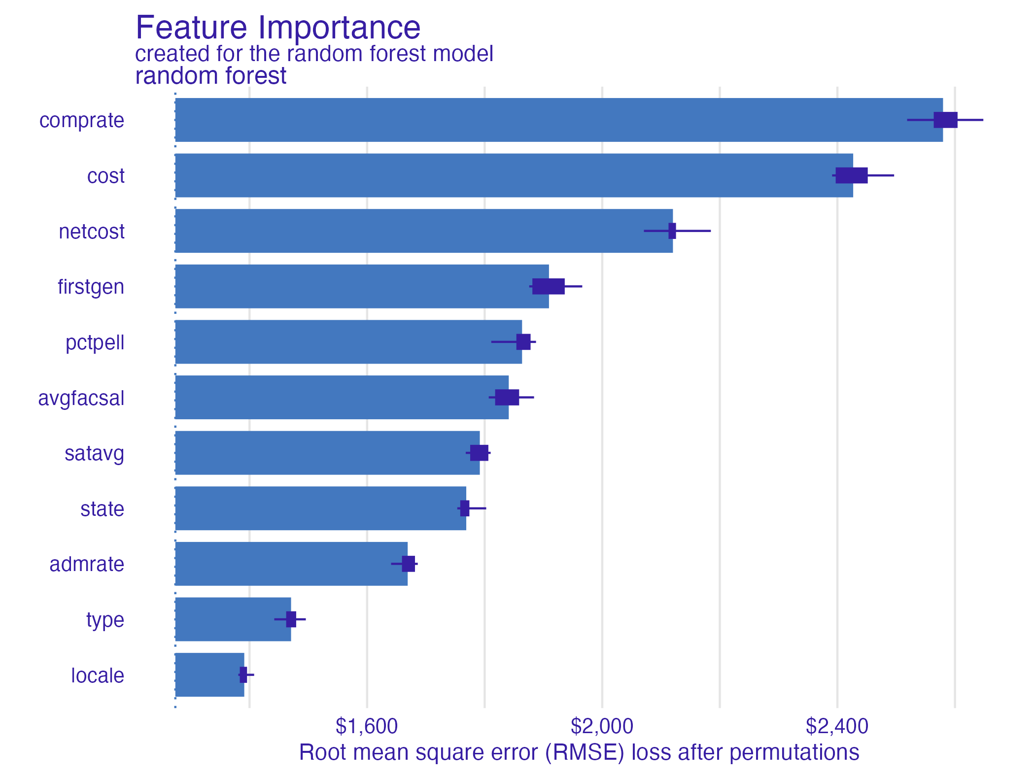
Permutation-based feature importance
Permutation-based feature importance
- Calculate the increase in the model’s prediction error after permuting the feature
- Randomly shuffle the feature’s values across observations
- Important feature
- Unimportant feature
For any given loss function do
1: compute loss function for original model
2: for variable i in {1,...,p} do
| randomize values
| apply given ML model
| estimate loss function
| compute feature importance (permuted loss / original loss)
end
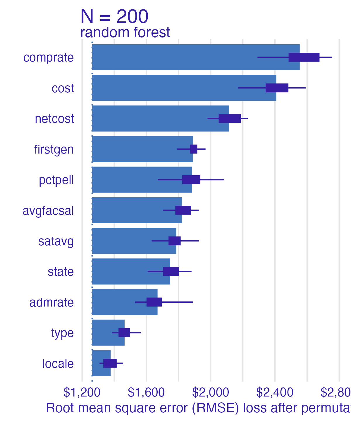
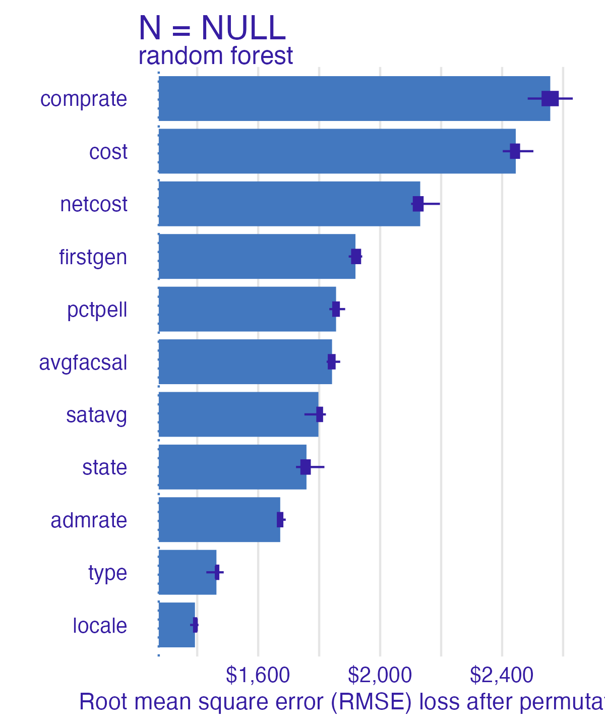
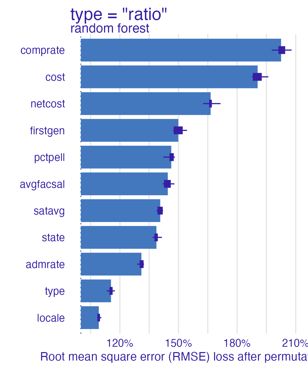
3. Sort variables by descending feature importance Random forest feature importance
Number of observations permuted
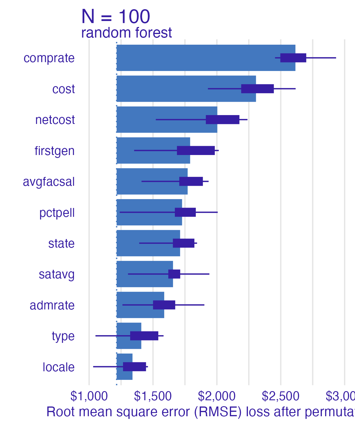
Measuring changes
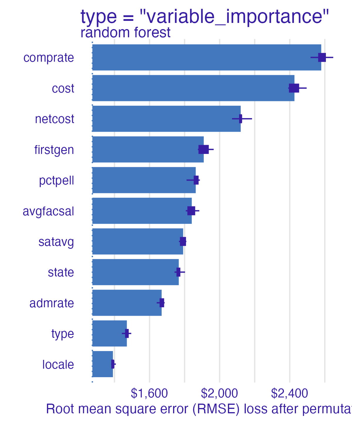
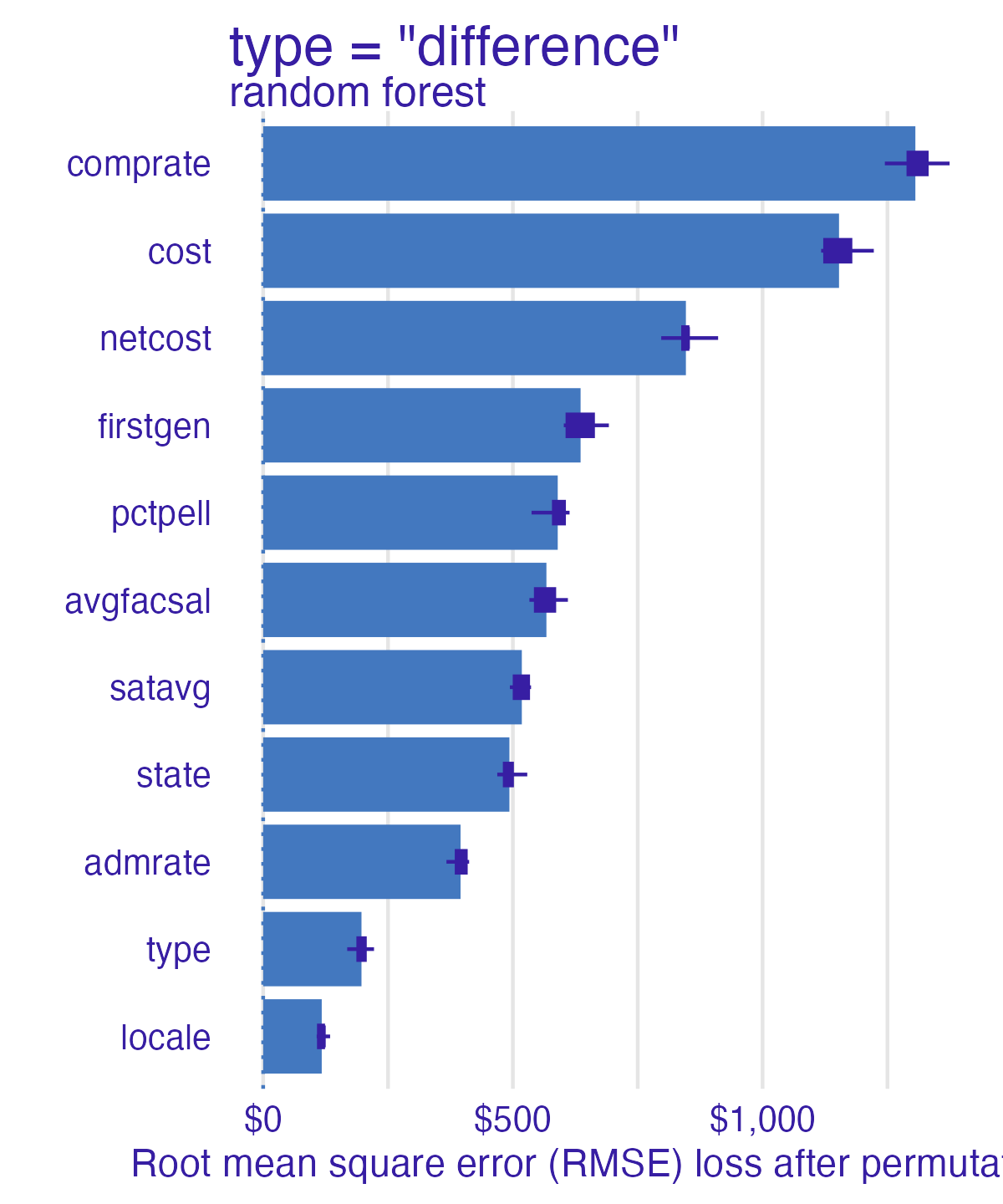
Compare all models
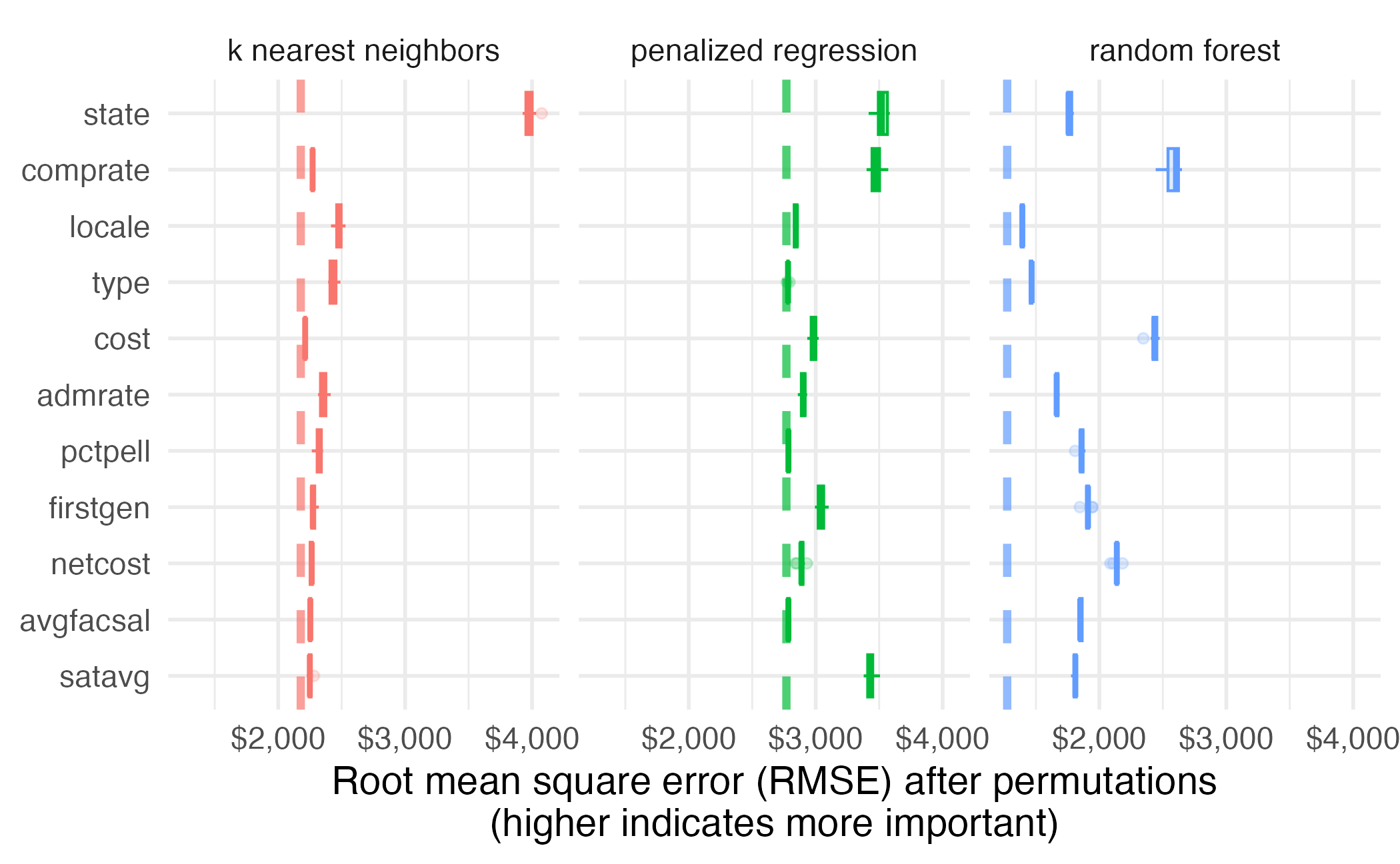
Permutation-based feature importance
Advantages
- Clear interpretation
- Succinct measure
- Does not require retraining the model
- Takes into account all interactions
Disadvantages
- Permutation adds randomness to results - results may vary greatly
- Computationally expensive
- Linked to the error of the model
- Need access to the true outcome
- Takes into account all interactions
Your Turn
- Review the DALEX code to estimate permutation-based feature importance for the debt prediction models
- Estimate permutation-based feature importance for the debt prediction models
- Interpret the resulting statistics - which features are most/least important? How does the model choice influence the results?
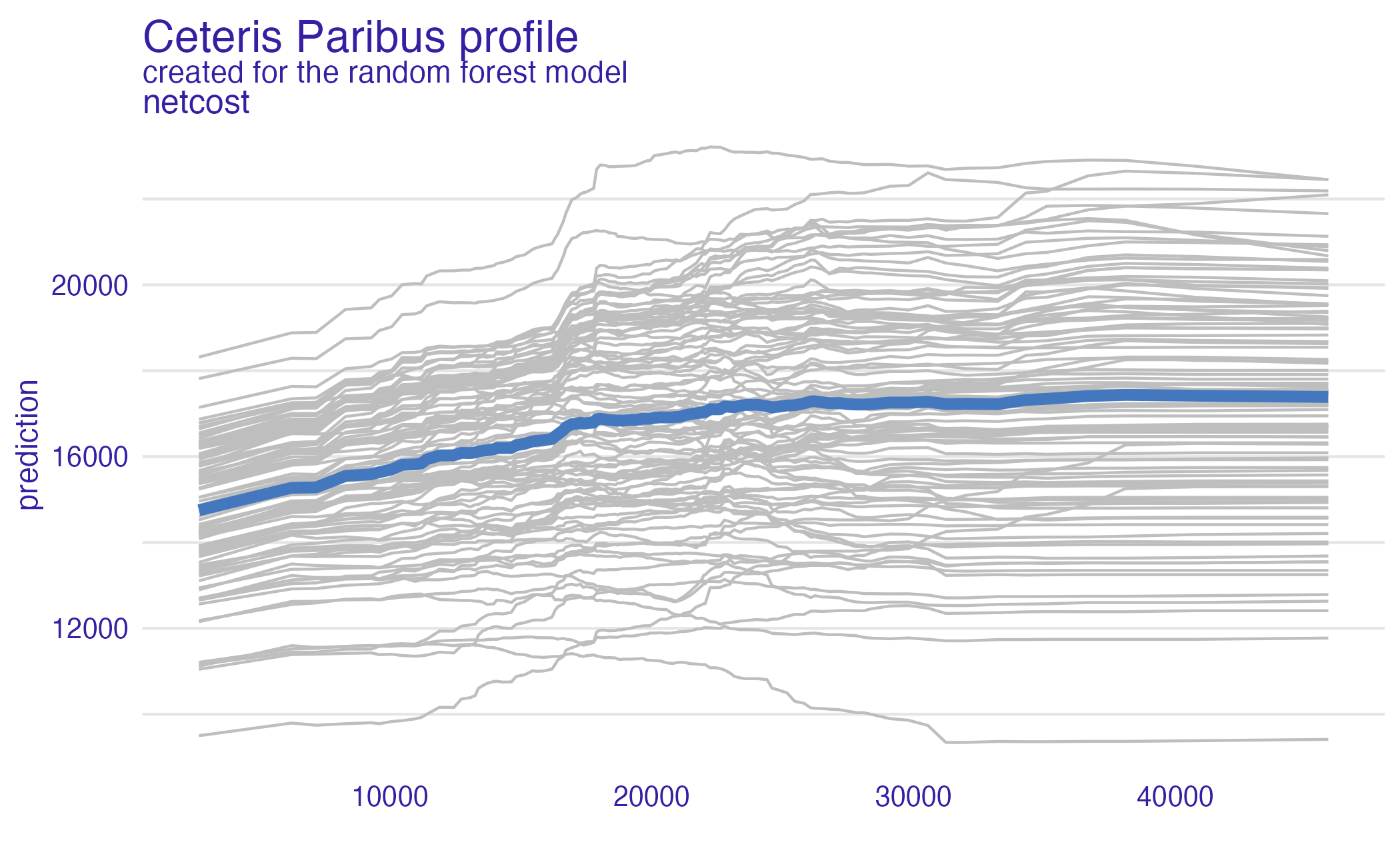
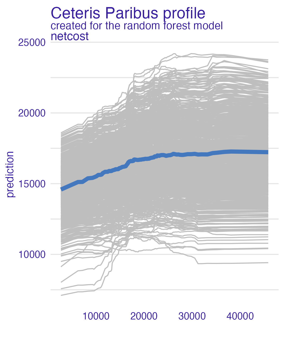
Partial dependence plot (PDP)
Individual conditional expectation (ICE)
- Ceteris peribus - “other things held constant”
- Marginal effect a feature has on the predictor
- Counterfactual comparison - what if this observation had \(Y\) value instead of \(X\)?
- Plot one observation that shows how the observation’s prediction changes when a feature changes
For a selected predictor (x)
1. Construct a grid of j evenly spaced values across the distribution
   of x: {x1, x2, ..., xj}
2. For i in {1,...,j} do
     | Copy the training data and replace the original values of x
       with the constant xi
     | Apply given ML model (i.e., obtain vector of predictions)
   End
3. Plot the predictions against x1, x2, ..., xj with lines connecting
   oberservations that correspond to the same row number in the original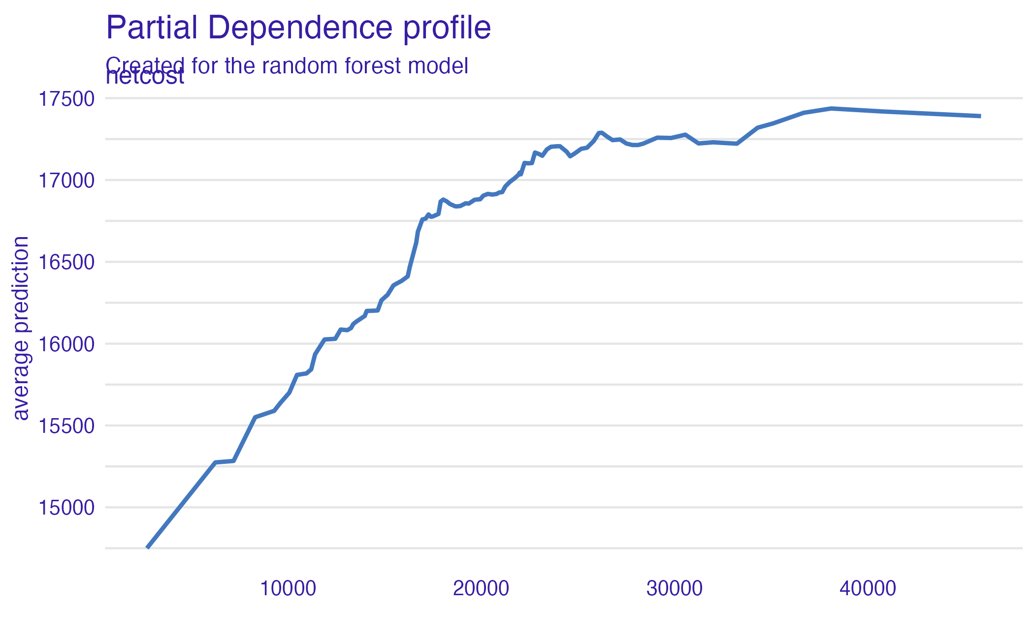
training dataPartial dependence plot (PDP)
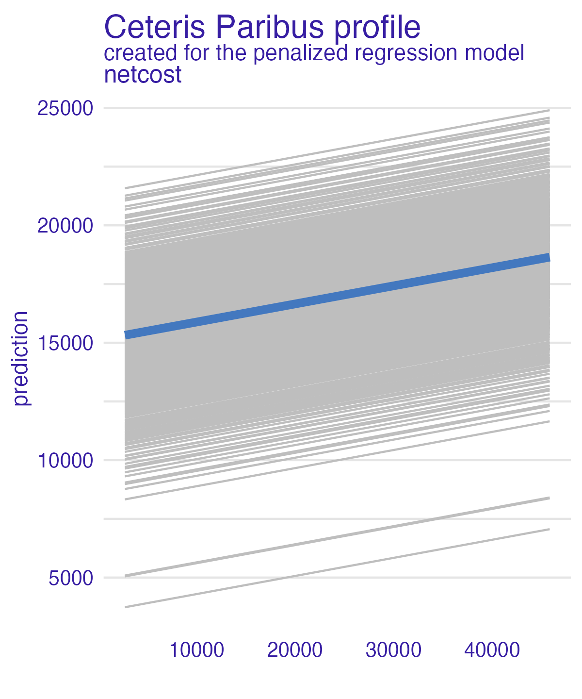
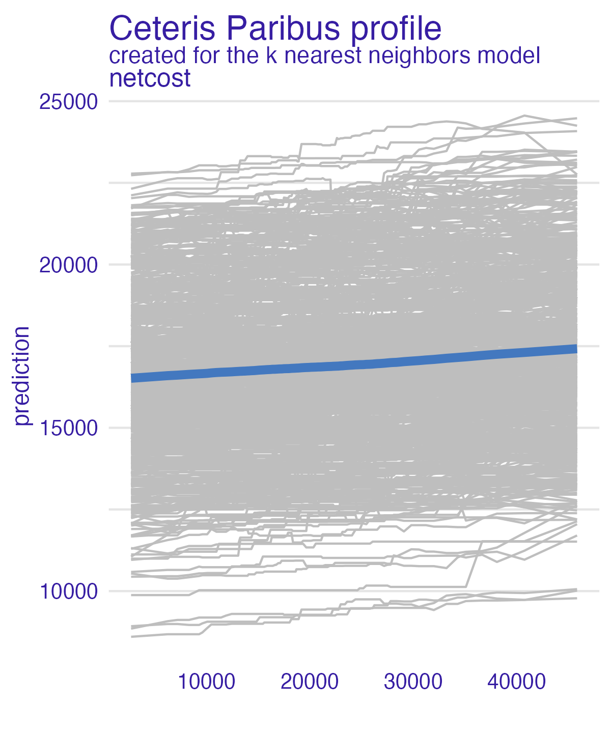
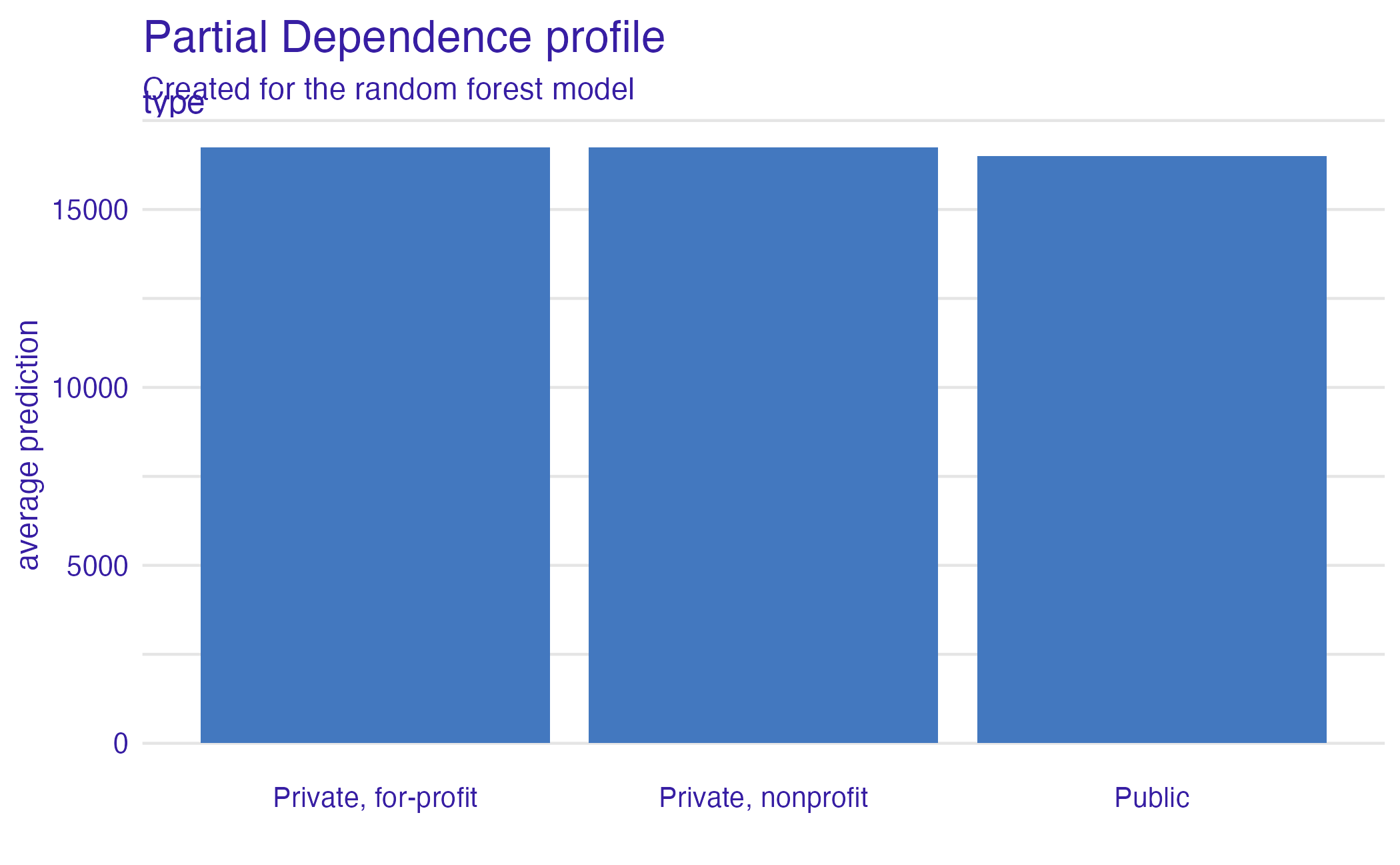
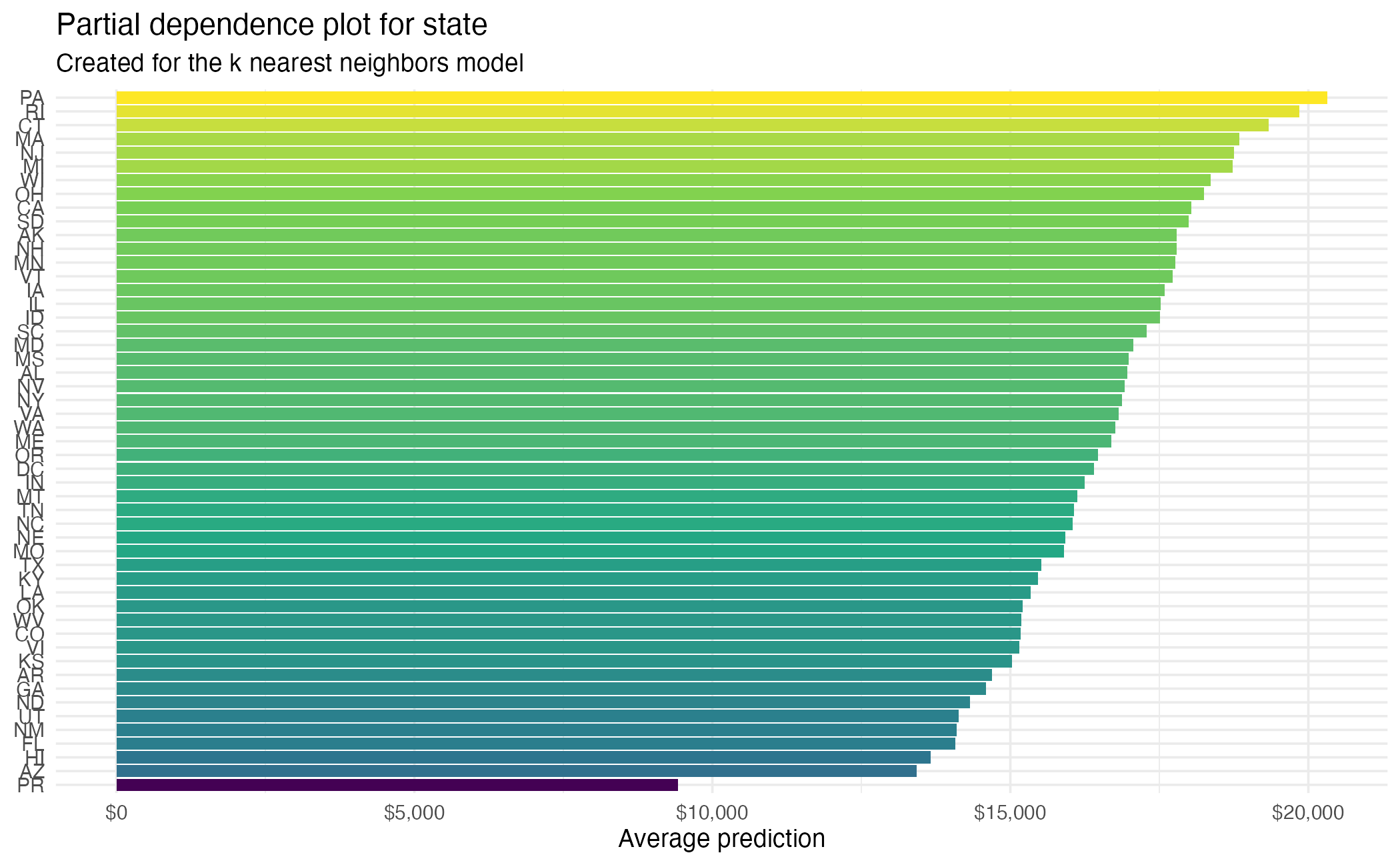
- Average multiple ICEs to estimate the marginal effect of a feature on the outcome of interest
For a selected predictor (x)
1. Construct a grid of j evenly spaced values across the distribution
   of x: {x1, x2, ..., xj}
2. For i in {1,...,j} do
     | Copy the training data and replace the original values of x
       with the constant xi
     | Apply given ML model (i.e., obtain vector of predictions)
     | Average predictions together
   End
3. Plot the averaged predictions against x1, x2, ..., xjNet cost (PDP)
Net cost (PDP + ICE)
Net cost (PDP + ICE) – all models
Type (PDP)
State (PDP)
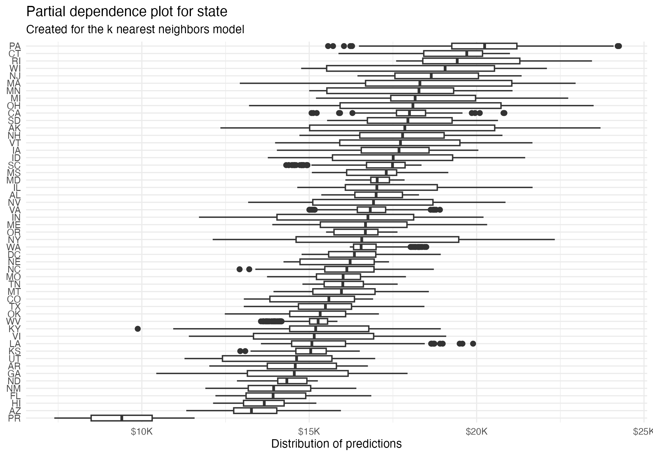
State (PDP + ICE)
Partial dependence plot (PDP)
Advantages
- Intuitive
- Clear interpretation (assuming variables are uncorrelated)
- Straightforward implementation
Disadvantages
- Limited to one or two variables
- Assumes independence of features
- Heterogeneous effects might be hidden - add ICE curves to visualize heterogeneity
Your Turn
- Review the DALEX code to estimate permutation-based feature importance for the debt prediction models
- Interpret how the average faculty salary influences the predictions of the debt models
Global surrogate
Global surrogate
- Use a white-box model to explain the predictions of a black-box model
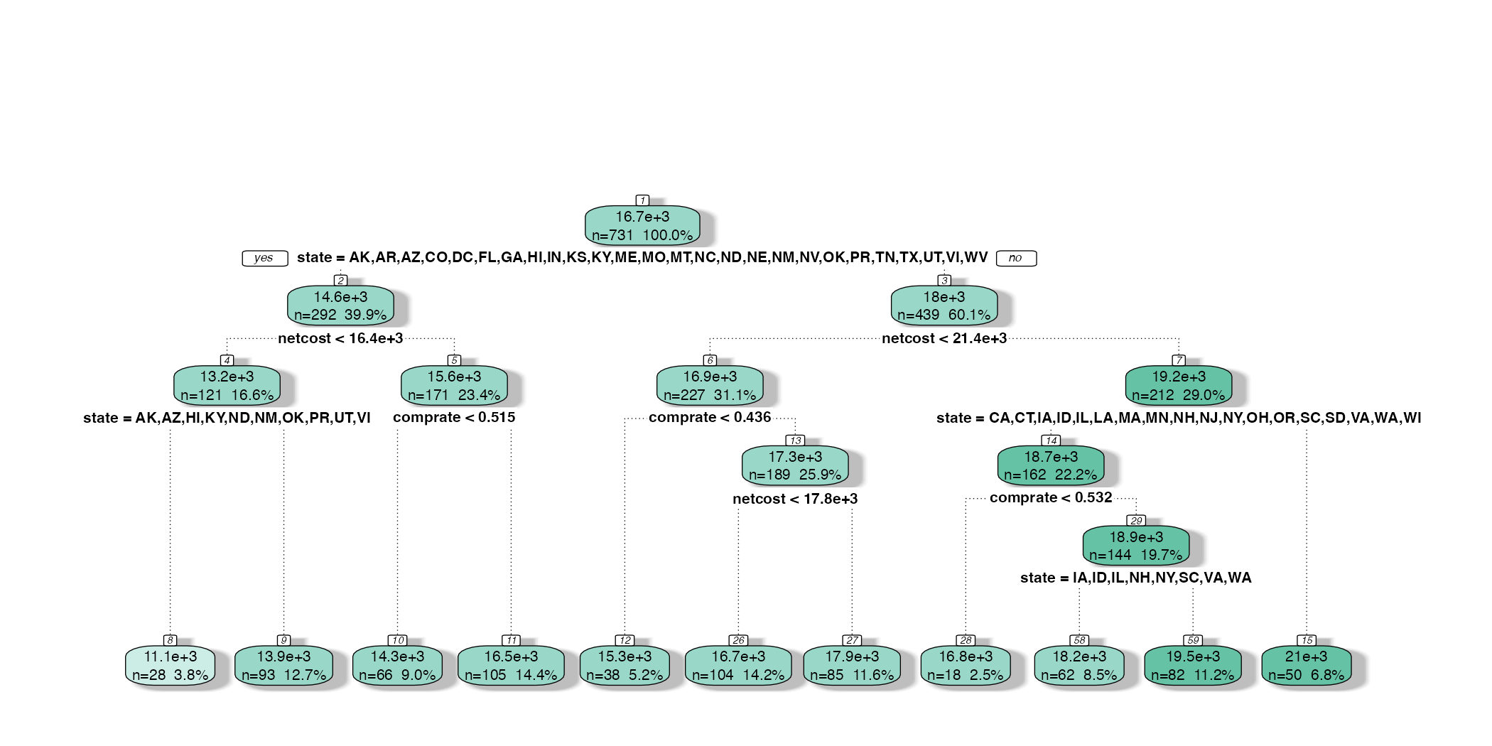
- Approximate the global results of a highly complex model with a naturally interpretable model (e.g. simple regression, decision tree)
- Use a metric such as \(R^2\) to evaluate the performance of the surrogate model
Global surrogate of the penalized regression model
Global surrogate \(R^2 = \text{73%}\)
Global surrogate
Advantages
- Flexible
- Intuitive
- Can assess the quality of the surrogate model
Disadvantages
- Drawing conclusions about the model, not the data
- How good is good enough for the surrogate?
Your Turn
- Review the code to fit a global surrogate model
- Interpret the nearest neighbors model using a decision tree surrogate model
Wrap-up
Wrap-up
- Interpretability is crucial for understanding and trusting machine learning models
- Permutation-based feature importance provides insight into the importance of features in a model
- Partial dependence plots provide a global view of the relationship between a feature and the model’s predictions
- Global surrogates approximate the predictions of a complex model with a simpler, interpretable model
Additional resources
- Interpretable Machine Learning: A Guide for Making Black Box Models Explainable by Christoph Molnar
- Explanatory Model Analysis by Przemyslaw Biecek and Tomasz Burzykowski