Tables
Lecture 22
April 25, 2023
# A tibble: 33 × 2
   field                                                           perc
   <chr>                                                          <dbl>
 1 Agriculture and natural resources                          0.0191
 2 Architecture and related services                          0.00480
 3 Area, ethnic, cultural, gender, and group studies          0.00411
 4 Biological and biomedical sciences                         0.0580
 5 Business                                                   0.192
 6 Communication, journalism, and related programs            0.0478
 7 Communications technologies                                0.00271
 8 Computer and information sciences                          0.0314
 9 Education                                                  0.0484
10 Engineering                                                0.0516
11 Engineering technologies                                   0.00910
12 English language and literature/letters                    0.0242
13 Family and consumer sciences/human sciences                0.0130
14 Foreign languages, literatures, and linguistics            0.0103
15 Health professions and related programs                    0.114
16 Homeland security, law enforcement, and firefighting       0.0331
17 Legal professions and studies                              0.00233
18 Liberal arts and sciences, general studies, and humanities 0.0230
19 Library science                                            0.0000522
20 Mathematics and statistics                                 0.0115
21 Military technologies and applied sciences                 0.000146
22 Multi/interdisciplinary studies                            0.0251
23 Parks, recreation, leisure, and fitness studies            0.0259
24 Philosophy and religious studies                           0.00584
25 Physical sciences and science technologies                 0.0159
26 Precision production                                       0.0000253
27 Psychology                                                 0.0620
28 Public administration and social services                  0.0181
29 Social sciences and history                                0.0881
30 Theology and religious vocations                           0.00512
31 Transportation and materials moving                        0.00249
32 Visual and performing arts                                 0.0506
33 Not classified by field of study 0 
# A tibble: 33 × 2
   field                                                           perc
   <chr>                                                          <dbl>
 1 Business                                                   0.192
 2 Health professions and related programs                    0.114
 3 Social sciences and history                                0.0881
 4 Psychology                                                 0.0620
 5 Biological and biomedical sciences                         0.0580
 6 Engineering                                                0.0516
 7 Visual and performing arts                                 0.0506
 8 Education                                                  0.0484
 9 Communication, journalism, and related programs            0.0478
10 Homeland security, law enforcement, and firefighting       0.0331
11 Computer and information sciences                          0.0314
12 Parks, recreation, leisure, and fitness studies            0.0259
13 Multi/interdisciplinary studies                            0.0251
14 English language and literature/letters                    0.0242
15 Liberal arts and sciences, general studies, and humanities 0.0230
16 Agriculture and natural resources                          0.0191
17 Public administration and social services                  0.0181
18 Physical sciences and science technologies                 0.0159
19 Family and consumer sciences/human sciences                0.0130
20 Mathematics and statistics                                 0.0115
21 Foreign languages, literatures, and linguistics            0.0103
22 Engineering technologies                                   0.00910
23 Philosophy and religious studies                           0.00584
24 Theology and religious vocations                           0.00512
25 Architecture and related services                          0.00480
26 Area, ethnic, cultural, gender, and group studies          0.00411
27 Communications technologies                                0.00271
28 Transportation and materials moving                        0.00249
29 Legal professions and studies                              0.00233
30 Military technologies and applied sciences                 0.000146
31 Library science                                            0.0000522
32 Precision production                                       0.0000253
33 Not classified by field of study 0 
| Field | Percentage |
|---|---|
| Business | 19.2% |
| Health professions and related programs | 11.4% |
| Social sciences and history | 8.8% |
| Psychology | 6.2% |
| Biological and biomedical sciences | 5.8% |
| Engineering | 5.2% |
| Visual and performing arts | 5.1% |
| Education | 4.8% |
| Communication, journalism, and related programs | 4.8% |
| Homeland security, law enforcement, and firefighting | 3.3% |
| Computer and information sciences | 3.1% |
| Parks, recreation, leisure, and fitness studies | 2.6% |
| Multi/interdisciplinary studies | 2.5% |
| English language and literature/letters | 2.4% |
| Liberal arts and sciences, general studies, and humanities | 2.3% |
| Agriculture and natural resources | 1.9% |
| Public administration and social services | 1.8% |
| Physical sciences and science technologies | 1.6% |
| Family and consumer sciences/human sciences | 1.3% |
| Mathematics and statistics | 1.2% |
| Foreign languages, literatures, and linguistics | 1.0% |
| Engineering technologies | 0.9% |
| Philosophy and religious studies | 0.6% |
| Theology and religious vocations | 0.5% |
| Architecture and related services | 0.5% |
| Area, ethnic, cultural, gender, and group studies | 0.4% |
| Communications technologies | 0.3% |
| Transportation and materials moving | 0.2% |
| Legal professions and studies | 0.2% |
| Military technologies and applied sciences | 0.0% |
| Library science | 0.0% |
| Precision production | 0.0% |
| Not classified by field of study | 0.0% |

Or in a plot?

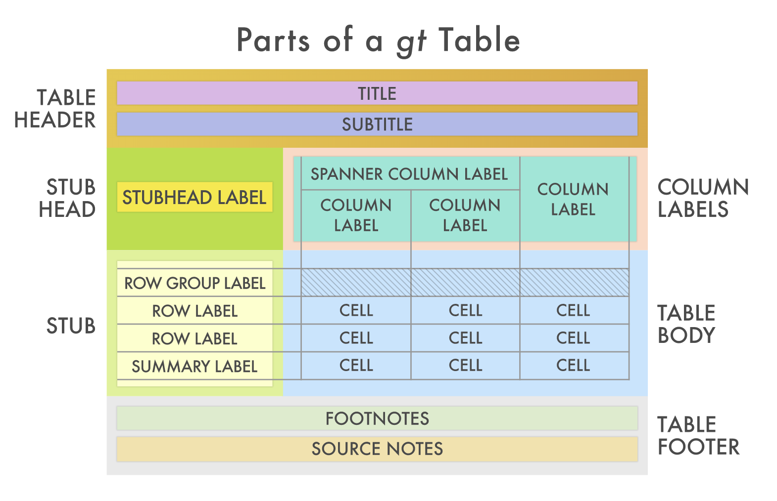
Tables with gt
We will use the gt (Grammar of Tables) package to create tables in R.
The gt philosophy: we can construct a wide variety of useful tables with a cohesive set of table parts.
Source: gt.rstudio.com
Should these data be displayed in a table or a plot?
| Popular Bachelor's degrees over the years | ||||||||||||||||||
|---|---|---|---|---|---|---|---|---|---|---|---|---|---|---|---|---|---|---|
| Field | 1971 | 1976 | 1981 | 1986 | 1991 | 1996 | 2001 | 2005 | 2006 | 2007 | 2008 | 2009 | 2010 | 2011 | 2012 | 2013 | 2014 | 2015 |
| Business | 14% | 15% | 21% | 24% | 23% | 19% | 21% | 22% | 21% | 21% | 21% | 22% | 22% | 21% | 20% | 20% | 19% | 19% |
| Health professions | 3% | 6% | 7% | 7% | 5% | 7% | 6% | 6% | 6% | 7% | 7% | 8% | 8% | 8% | 9% | 10% | 11% | 11% |
| Social sciences and history | 18% | 14% | 11% | 9% | 11% | 11% | 10% | 11% | 11% | 11% | 11% | 11% | 10% | 10% | 10% | 10% | 9% | 9% |
| Other | 65% | 65% | 61% | 60% | 60% | 62% | 62% | 62% | 62% | 61% | 61% | 60% | 60% | 60% | 60% | 61% | 61% | 61% |


Add visualizations to your table
Example: Add sparklines to display trend alongside raw data
| Popular Bachelor's degrees over the years | |||||||||||||||||||
|---|---|---|---|---|---|---|---|---|---|---|---|---|---|---|---|---|---|---|---|
| Field | Trend | 1971 | 1976 | 1981 | 1986 | 1991 | 1996 | 2001 | 2005 | 2006 | 2007 | 2008 | 2009 | 2010 | 2011 | 2012 | 2013 | 2014 | 2015 |
| Business |  |
14% | 15% | 21% | 24% | 23% | 19% | 21% | 22% | 21% | 21% | 21% | 22% | 22% | 21% | 20% | 20% | 19% | 19% |
| Health professions |  |
3% | 6% | 7% | 7% | 5% | 7% | 6% | 6% | 6% | 7% | 7% | 8% | 8% | 8% | 9% | 10% | 11% | 11% |
| Social sciences and history |  |
18% | 14% | 11% | 9% | 11% | 11% | 10% | 11% | 11% | 11% | 11% | 11% | 10% | 10% | 10% | 10% | 9% | 9% |
| Other |  |
65% | 65% | 61% | 60% | 60% | 62% | 62% | 62% | 62% | 61% | 61% | 60% | 60% | 60% | 60% | 61% | 61% | 61% |
Custom function with ggplot()

Basic gt table with sparklines
BA_degrees_other |>
  pivot_wider(names_from = year, values_from = perc) |>
mutate(ggplot = NA, .after = field) |>
gt() |>
text_transform(
locations = cells_body(columns = ggplot),
fn = function(x) {
map(
.x = BA_degrees_other_plots$plot, .f = ggplot_image,
height = px(15), aspect_ratio = 4
)
}
)| field | ggplot | 1971 | 1976 | 1981 | 1986 | 1991 | 1996 | 2001 | 2005 | 2006 | 2007 | 2008 | 2009 | 2010 | 2011 | 2012 | 2013 | 2014 | 2015 |
|---|---|---|---|---|---|---|---|---|---|---|---|---|---|---|---|---|---|---|---|
| Business |  |
0.13742036 | 0.15465473 | 0.21442886 | 0.23961783 | 0.22764399 | 0.19456092 | 0.2117997 | 0.2164815 | 0.21413480 | 0.21490238 | 0.21448445 | 0.21734496 | 0.21705247 | 0.21277490 | 0.20491161 | 0.19609363 | 0.19149908 | 0.19198505 |
| Health professions |  |
0.03003704 | 0.05820711 | 0.06808072 | 0.06611407 | 0.05470345 | 0.07390762 | 0.0610310 | 0.0560599 | 0.06192459 | 0.06680043 | 0.07131995 | 0.07519675 | 0.07856325 | 0.08360056 | 0.09132819 | 0.09843016 | 0.10628934 | 0.11410846 |
| Social sciences and history |  |
0.18496898 | 0.13653421 | 0.10748444 | 0.09499678 | 0.11430119 | 0.10858505 | 0.1029087 | 0.1090085 | 0.10872639 | 0.10772512 | 0.10707333 | 0.10523111 | 0.10472150 | 0.10324215 | 0.09961929 | 0.09659250 | 0.09257653 | 0.08810017 |
| Other |  |
0.64757362 | 0.65060395 | 0.61000599 | 0.59927133 | 0.60335137 | 0.62294641 | 0.6242607 | 0.6184501 | 0.61521422 | 0.61057207 | 0.60712227 | 0.60222718 | 0.59966277 | 0.60038239 | 0.60414092 | 0.60888370 | 0.60963506 | 0.60580632 |
Generate the table
| Popular Bachelor's degrees over the years | |||||||||||||||||||
|---|---|---|---|---|---|---|---|---|---|---|---|---|---|---|---|---|---|---|---|
| Field | Trend | 1971 | 1976 | 1981 | 1986 | 1991 | 1996 | 2001 | 2005 | 2006 | 2007 | 2008 | 2009 | 2010 | 2011 | 2012 | 2013 | 2014 | 2015 |
| Business | |
14% | 15% | 21% | 24% | 23% | 19% | 21% | 22% | 21% | 21% | 21% | 22% | 22% | 21% | 20% | 20% | 19% | 19% |
| Health professions | |
3% | 6% | 7% | 7% | 5% | 7% | 6% | 6% | 6% | 7% | 7% | 8% | 8% | 8% | 9% | 10% | 11% | 11% |
| Social sciences and history | |
18% | 14% | 11% | 9% | 11% | 11% | 10% | 11% | 11% | 11% | 11% | 11% | 10% | 10% | 10% | 10% | 9% | 9% |
| Other | |
65% | 65% | 61% | 60% | 60% | 62% | 62% | 62% | 62% | 61% | 61% | 60% | 60% | 60% | 60% | 61% | 61% | 61% |
Adding color text
| Popular Bachelor's degrees over the years | |||||||||||||||||||
|---|---|---|---|---|---|---|---|---|---|---|---|---|---|---|---|---|---|---|---|
| Field | Trend | 1971 | 1976 | 1981 | 1986 | 1991 | 1996 | 2001 | 2005 | 2006 | 2007 | 2008 | 2009 | 2010 | 2011 | 2012 | 2013 | 2014 | 2015 |
| Business | |
14% | 15% | 21% | 24% | 23% | 19% | 21% | 22% | 21% | 21% | 21% | 22% | 22% | 21% | 20% | 20% | 19% | 19% |
| Health professions | |
3% | 6% | 7% | 7% | 5% | 7% | 6% | 6% | 6% | 7% | 7% | 8% | 8% | 8% | 9% | 10% | 11% | 11% |
| Social sciences and history | |
18% | 14% | 11% | 9% | 11% | 11% | 10% | 11% | 11% | 11% | 11% | 11% | 10% | 10% | 10% | 10% | 9% | 9% |
| Other | |
65% | 65% | 61% | 60% | 60% | 62% | 62% | 62% | 62% | 61% | 61% | 60% | 60% | 60% | 60% | 61% | 61% | 61% |
plot_spark_color <- function(df) {
ggplot(df, aes(x = year, y = perc, color = line_color)) +
geom_line(size = 20) +
theme_void() +
scale_color_identity()
}
BA_degrees_other_plots_color <- BA_degrees_other |>
mutate(line_color = case_when(
field == "Business" ~ "#9D6C06",
field == "Health professions" ~ "#077DAA",
field == "Social sciences and history" ~ "#026D4E",
field == "Other" ~ "#A39A09"
)) |>
nest(field_df = c(year, perc, line_color)) |>
mutate(plot = map(field_df, plot_spark_color))
BA_degrees_other |>
  pivot_wider(names_from = year, values_from = perc) |>
  mutate(ggplot = NA, .after = field) |>
gt() |>
text_transform(
locations = cells_body(columns = ggplot),
fn = function(x) {
map(BA_degrees_other_plots_color$plot, ggplot_image, height = px(15), aspect_ratio = 4)
}
) |>
cols_width(ggplot ~ px(100)) |>
cols_align(align = "left", columns = field) |>
fmt_percent(columns = where(is.numeric), decimals = 0) |>
tab_style(style = cell_text(color = "#9D6C06"), locations = cells_body(rows = 1, columns = field)) |>
tab_style(style = cell_text(color = "#077DAA"), locations = cells_body(rows = 2, columns = field)) |>
tab_style(style = cell_text(color = "#026D4E"), locations = cells_body(rows = 3, columns = field)) |>
tab_style(style = cell_text(color = "#A39A09"), locations = cells_body(rows = 4, columns = field)) |>
cols_label(field = "Field", ggplot = "Trend") |>
tab_spanner(label = "Popular Bachelor's degrees over the years", columns = everything()) |>
tab_style(style = cell_text(weight = "bold"), locations = cells_column_spanners())Other packages
knitr::kable(): “Cheapest” pretty tables in Quarto
- Other (than HTML) outputs:
- LaTeX/PDF: kableExtra
- Word: flextable
- gtsummary: For summarizing statistical output with gt
- Creating beautiful tables in R with {gt}
