Interactive reporting with Shiny (I)
Lecture 22
Dr. Benjamin Soltoff
Cornell University
INFO 3312/5312 - Spring 2026
April 16, 2026
Announcements
Announcements
- Finish homework 05
- Project 02 drafts
- Remaining class schedule
Learning objectives
- Introduce Shiny for interactive web applications
- Review implementation of basic Shiny app
- Introduce reactive programming concepts
Application exercise
ae-21
Instructions
- Go to the course GitHub org and find your
ae-21(repo name will be suffixed with your GitHub name). - Clone the repo in Positron, run
renv::restore()to install the required packages, open the Quarto document in the repo, and follow along and complete the exercises. - Render, commit, and push your edits by the AE deadline – end of the day
Communicating interactively with data
- Interactive charts
- Scrollytelling
- Dashboards
- Interactive web applications
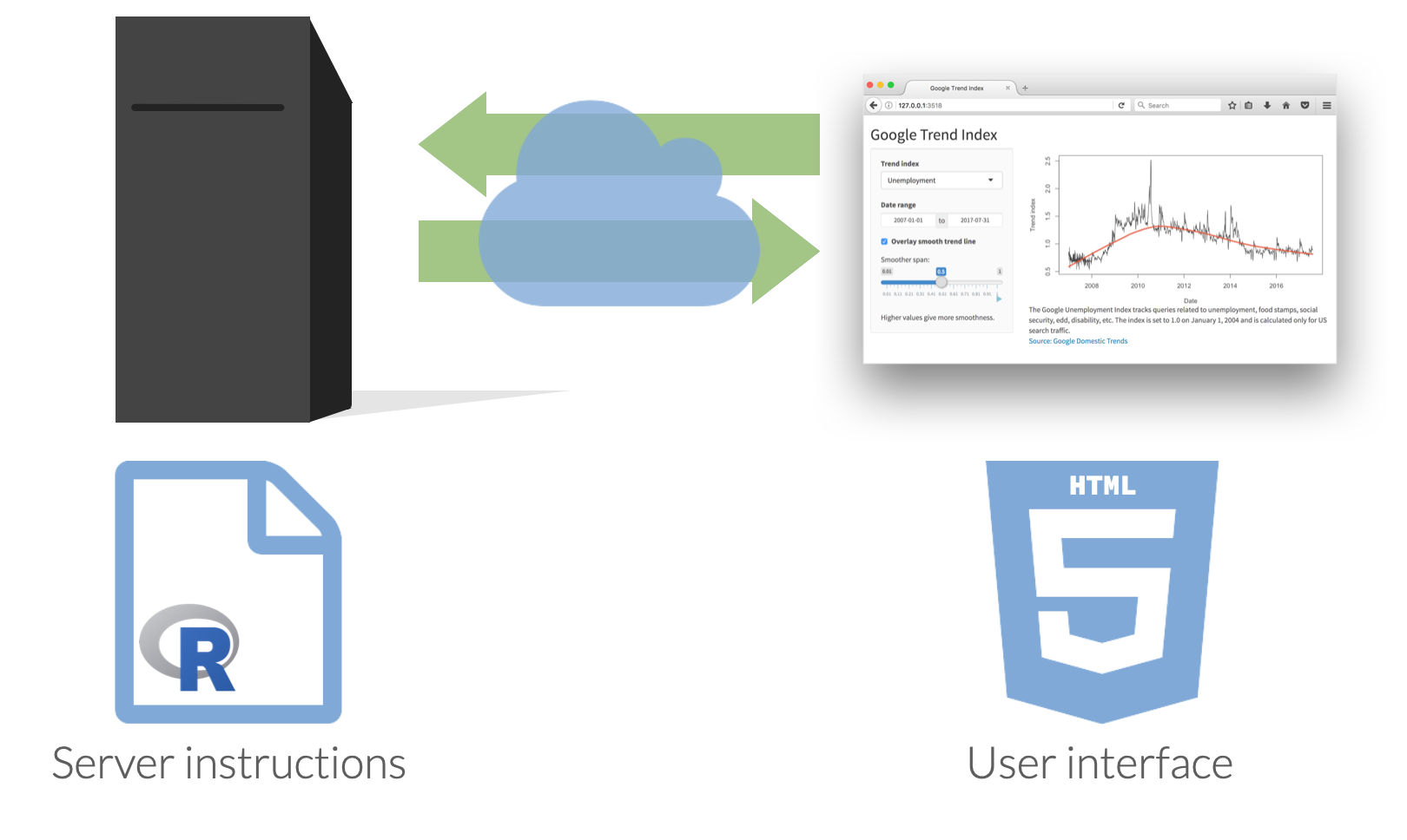
Shiny: High level view
Every Shiny app has a webpage that the user visits,
and behind this webpage there is a computer that serves this webpage by running R (or Python!).
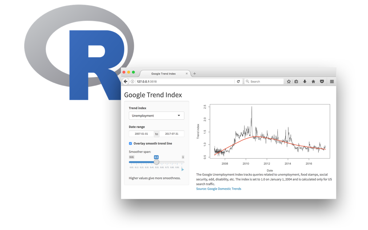
When running your app locally, the computer serving your app is your computer.
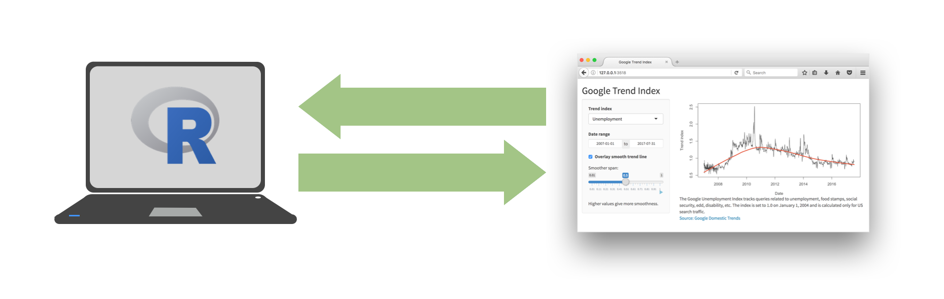
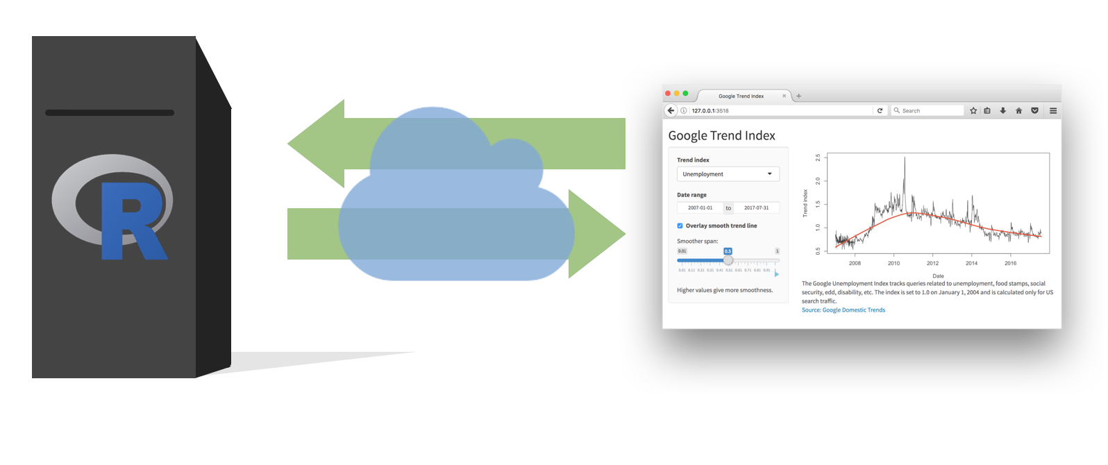
When your app is deployed, the computer serving your app is a web server.
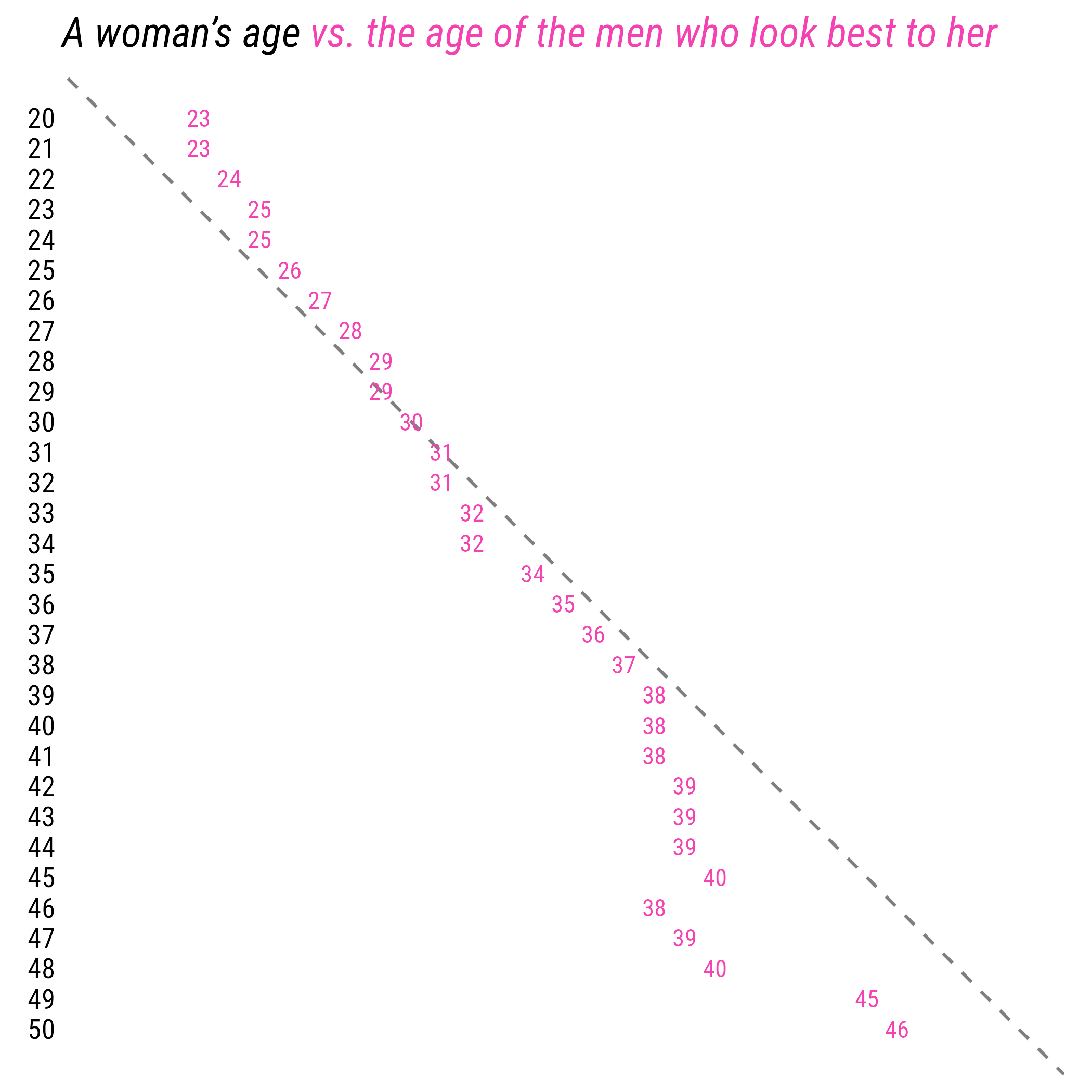
Dating rules
Age gaps
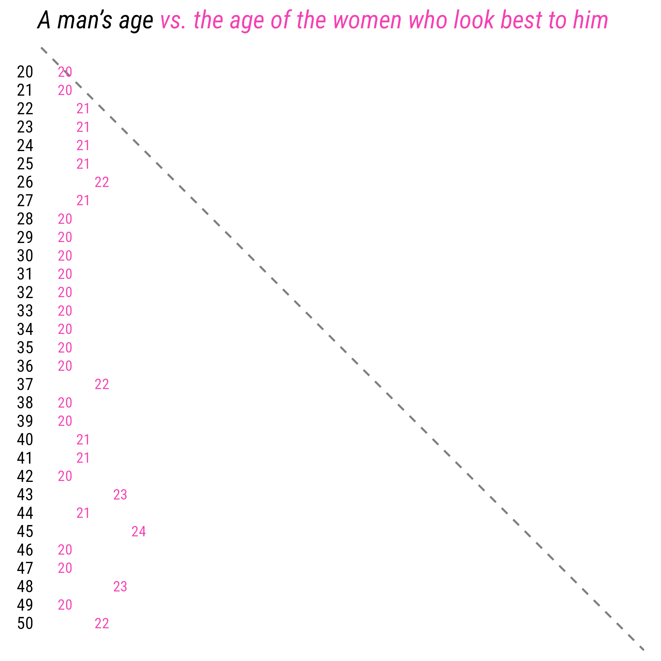
Source: Chapter 1 - Dataclysm, by Christian Rudder
Dating rules
Anatomy of a Shiny app
Shiny
- Shiny is a web application framework for R (and Python) that allows you to build interactive web applications using R (or Python) code
- Host standalone apps on a webpage, embed them in Quarto documents, or build dashboards
- Extend Shiny apps with CSS themes, {htmlwidgets}, and JavaScript actions

Learn more at https://shiny.posit.co/
{bslib}
Modern UI toolkit for Shiny based on Bootstrap
Creation of delightful and customizable Shiny dashboards with cards, value boxes, sidebars, etc.
Use of modern versions of Bootstrap and Bootswatch

Learn more at https://rstudio.github.io/bslib
Shiny + {bslib}
is now the officially recommended way to build Shiny apps.
- {shiny} functions uses
camelCase - {bslib} functions use
snake_case
App components
Every Shiny app has two main components:
A UI (user interface) which controls how the app looks
and a server function which controls how the app works.
Weather data
# A tibble: 23,376 × 17
id name airport_code country state region longitude latitude date temp_avg temp_min
<dbl> <chr> <chr> <chr> <chr> <chr> <dbl> <dbl> <date> <dbl> <dbl>
1 72202 Miami KMIA US FL South -80.3 25.8 2022-01-01 24.2 21.1
2 72202 Miami KMIA US FL South -80.3 25.8 2022-01-02 24.4 21.7
3 72202 Miami KMIA US FL South -80.3 25.8 2022-01-03 22.7 17.8
4 72202 Miami KMIA US FL South -80.3 25.8 2022-01-04 20.4 16.7
5 72202 Miami KMIA US FL South -80.3 25.8 2022-01-05 22.9 19.4
6 72202 Miami KMIA US FL South -80.3 25.8 2022-01-06 21.4 16.7
7 72202 Miami KMIA US FL South -80.3 25.8 2022-01-07 23.6 20.6
# ℹ 23,369 more rows
# ℹ 6 more variables: temp_max <dbl>, precip <dbl>, snow <dbl>, wind_direction <dbl>,
# wind_speed <dbl>, air_press <dbl>Demo 01 - Our first app
demos/demo-01.R
library(tidyverse)
library(shiny)
library(bslib)
d <- read_csv(here::here("data/weather.csv"))
ui <- page_sidebar(
title = "Temperatures at Major Airports",
sidebar = sidebar(
radioButtons(
inputId = "name",
label = "Select an airport",
choices = c(
"Hartsfield-Jackson Atlanta",
"Raleigh-Durham",
"Denver",
"Los Angeles",
"John F. Kennedy"
)
)
),
plotOutput(outputId = "plot")
)
server <- function(input, output, session) {
output$plot <- renderPlot({
d |>
filter(name %in% input$name) |>
ggplot(mapping = aes(x = date, y = temp_avg)) +
geom_line()
})
}
shinyApp(ui = ui, server = server)⌨️ Your turn - exercise 01
Instructions
Open exercises/ex-01.R and execute it via the Run App button.
Check that you are able to successfully run the Shiny app and are able to interact with it by picking a new airport.
If everything is working, try modifying the code:
- Try adding or removing a city from
radioButtons() - Check what happens if you add a city that is not in
weather.csv(i.e. Ithaca)
04:00
UIs
Layouts
Shiny uses page layout functions as a way to specify the general organization of the UI of an app.
Our first app used a sidebar layout created with page_sidebar(). This layout consists of:
a
titlea
sidebar(which usually holds inputs or extra information)A collection of other Shiny UI elements which form the body of the app
This sidebar layout is a good place to start for most simple apps, but there are many other layouts that can be used to create more complex and interesting apps.
Shiny layouts
Shiny vs {bslib} layouts
Since page_sidebar() uses snake_case we can infer it is from {bslib}. If you’ve seen older Shiny code you may have seen fluidPage() + sidebarLayout() which come from {shiny}.
There are analogues of almost all of Shiny’s original page layouts in {bslib}, either choice is viable and will let you create a working Shiny app.
We have opted to use the {bslib} layouts because they are more modern and typically have a more user friendly (less nested) syntax.
UI functions are HTML
One of the neat tricks of Shiny is that the interface is just a webpage, and this can be seen by the fact that UI functions are just R functions that generate HTML.
We can run any of the following in our console and see the underlying HTML of each element.
<button id="id" type="button" class="btn btn-default action-button">
<span class="action-label">Click me!</span>
</button><div class="form-group shiny-input-container">
<label class="control-label" id="test-label" for="test">Test</label>
<div>
<select class="shiny-input-select form-control" id="test"><option value="A" selected>A</option>
<option value="B">B</option>
<option value="C">C</option></select>
</div>
</div><img src="shiny.png"/>Inputs and outputs
Shiny input widgets
Shiny inputs
⌨️ Your turn - exercise 02
Instructions
Starting from the code in exercises/ex-02.R try changing the radioButton() input to one of the following:
selectInput()withmultiple = FALSEselectInput()withmultiple = TRUEcheckboxGroupInput()
What happens? Does the app still work as expected?
06:00
Shiny output
| Function | Outputs |
|---|---|
plotOutput() |
plot |
tableOutput() |
table |
uiOutput() |
Shiny UI element |
textOutput() |
text |
- Plots, tables, text - anything that R creates and users see
- Initialize as empty placeholder space until object is created
Shiny output widgets
Basic reactivity
*Output() \(\rightarrow\) render*()
| Output function | Render function |
|---|---|
plotOutput() |
renderPlot({}) |
tableOutput() |
renderTable({}) |
uiOutput() |
renderUI({}) |
textOutput() |
renderText({}) |
Reactive elements
demos/demo-01.R
library(tidyverse)
library(shiny)
library(bslib)

d <- read_csv(here::here("data/weather.csv"))

ui <- page_sidebar(
  title = "Temperatures at Major Airports",
  sidebar = sidebar(
    radioButtons(
      inputId = "name",
      label = "Select an airport",
      choices = c(
        "Hartsfield-Jackson Atlanta",
        "Raleigh-Durham",
        "Denver",
        "Los Angeles",
        "John F. Kennedy"
      )
    )
  ),
  plotOutput(outputId = "plot")
)

server <- function(input, output, session) {
  output$plot <- renderPlot({
    d |>
      filter(name %in% input$name) |>
      ggplot(mapping = aes(x = date, y = temp_avg)) +
      geom_line()
  })
}

shinyApp(ui = ui, server = server)Our inputs and outputs are defined by the elements in our ui.
Reactive graph
demos/demo-01.R
library(tidyverse)
library(shiny)
library(bslib)

d <- read_csv(here::here("data/weather.csv"))

ui <- page_sidebar(
  title = "Temperatures at Major Airports",
  sidebar = sidebar(
    radioButtons(
      inputId = "name",
      label = "Select an airport",
      choices = c(
        "Hartsfield-Jackson Atlanta",
        "Raleigh-Durham",
        "Denver",
        "Los Angeles",
        "John F. Kennedy"
      )
    )
  ),
  plotOutput(outputId = "plot")
)

server <- function(input, output, session) {
  output$plot <- renderPlot({
    d |>
      filter(name %in% input$name) |>
      ggplot(mapping = aes(x = date, y = temp_avg)) +
      geom_line()
  })
}

shinyApp(ui = ui, server = server)The reactive logic is defined in our server() function - {shiny} takes care of figuring out what depends on what.
Demo 02 - adding an input
demos/demo-02.R
library(tidyverse)
library(shiny)
library(bslib)

d <- read_csv(here::here("data/weather.csv"))

d_vars <- c(
  "Average temp" = "temp_avg",
  "Min temp" = "temp_min",
  "Max temp" = "temp_max",
  "Total precip" = "precip",
  "Snow depth" = "snow",
  "Wind direction" = "wind_direction",
  "Wind speed" = "wind_speed",
  "Air pressure" = "air_press"
)

ui <- page_sidebar(
  title = "Weather Forecasts",
  sidebar = sidebar(
    radioButtons(
      inputId = "name",
      label = "Select an airport",
      choices = c(
        "Raleigh-Durham",
        "Houston Intercontinental",
        "Denver",
        "Los Angeles",
        "John F. Kennedy"
      )
    ),
    selectInput(
      inputId = "var",
      label = "Select a variable",
      choices = d_vars,
      selected = "temp_avg"
    )
  ),
  plotOutput(outputId = "plot")
)

server <- function(input, output, session) {
  output$plot <- renderPlot({
    d |>
      filter(name %in% input$name) |>
      ggplot(mapping = aes(x = date, y = .data[[input$var]])) +
      geom_line() +
      labs(title = str_c(input$name, "-", input$var))
  })
}

shinyApp(ui = ui, server = server)
.data pronoun
A useful feature from {rlang} that can be used across much of the {tidyverse} to reference columns in a data frame using a variable.
This helps avoid some of the complexity around “non-standard evaluation” (e.g. {{, !!, enquo(), etc.) when working with functions built with tidyeval (e.g. {dplyr} and {ggplot2}).
More information: .data and .env pronouns
Reactive graph
With these additions, what does our reactive graph look like now?
⌨️ Your turn - exercise 03
Instructions
Starting with the code in exercises/ex-03.R (based on demo-02.R’s code) add a tableOutput() with the id minmax to the app’s body.
Once you have done that, you should then add logic to the server() function to render the table so that it shows the min and max average temperature for each year contained in the data.
- You will need to add an appropriate output in the
ui - And a corresponding reactive expression in the
server()function to generate these summaries. lubridate::year()will be useful along withdplyr::summarize().
10:00
Wrap-up
Wrap-up
- Shiny is a powerful tool for building interactive web applications with R, and {bslib} provides a modern and flexible way to design the UI of these apps
- Reactive programming is a key concept in Shiny that allows for dynamic and responsive applications
- Understanding how to use
reactive()and observers is essential for building effective Shiny apps
Acknowledgements
- Slides derived in part from posit::conf 2025 - Shiny for R Workshop by Colin Rundel and licensed under a Creative Commons Attribution 4.0 International License.
