| Characteristic | Beta | 95% CI1 | p-value |
|---|---|---|---|
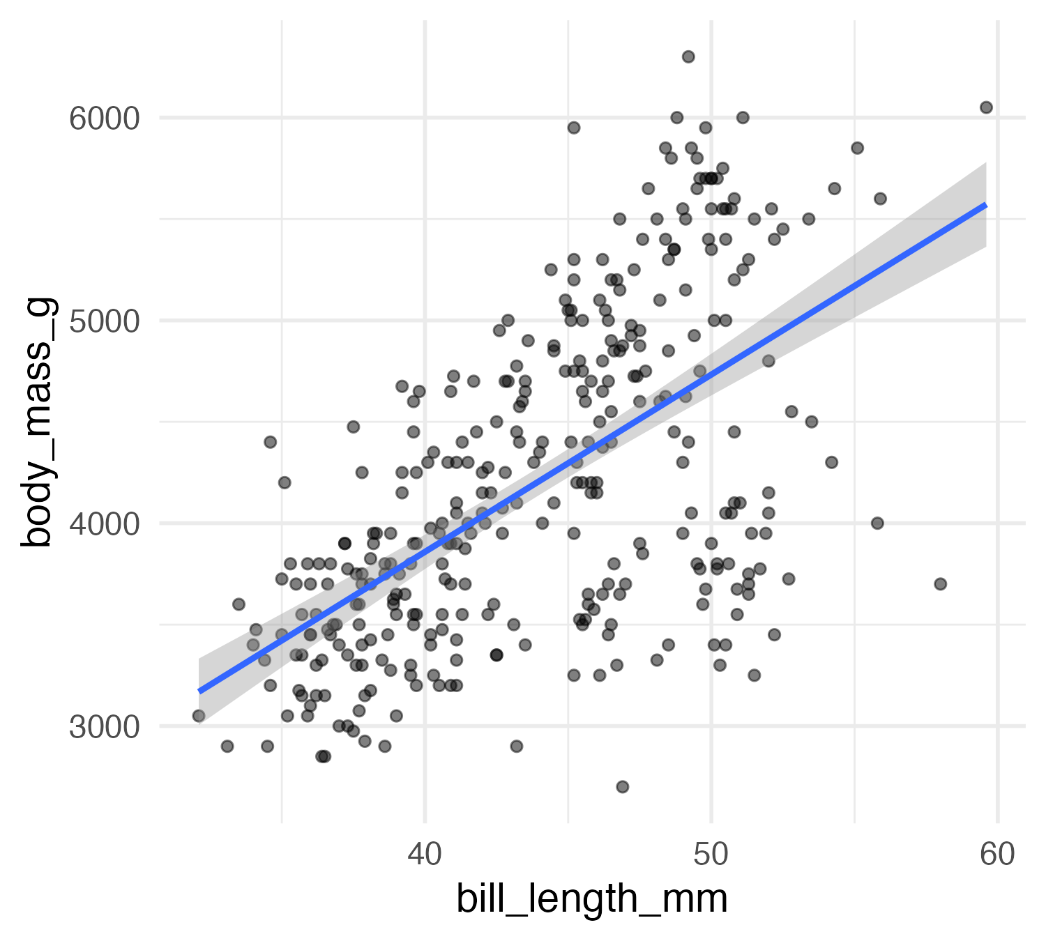
| bill_length_mm | 87 | 75, 100 | <0.001 |
| 1 CI = Confidence Interval | |||
Interpretable machine learning: overview and regression models
Lecture 22
Dr. Benjamin Soltoff
Cornell University
INFO 3312/5312 - Spring 2025
April 18, 2024
Announcements
Announcements
- Homework 06
- Friday lab: work on team projects
Goals
- Introduce the concepts of interpretability and explainability
- Identify points of interpretation in regression-based approaches
- Communicate predictions, comparisons, and slopes of regression models
- Distinguish between different forms of marginal effects
Interpretability and explainability
Interpretation
- Interpretability is the degree to which a human can understand the cause of a decision
- Interpretability is the degree to which a human can consistently predict the model’s result
- How does this model work?
Explanation
Answer to the “why” question
- Why did the government collapse?
- Why was my loan rejected?
- Focuses on a single prediction
What is a good explanation?
- Contrastive: why was this prediction made instead of another prediction?
- Selected: Focuses on just a handful of reasons, even if the problem is more complex
- Social: Needs to be understandable by your audience
- Truthful: Explanation should predict the event as truthfully as possible
- Generalizable: Explanation could apply to many predictions
Global vs. local methods
- Interpretation \(\leadsto\) global methods
- Explanation \(\leadsto\) local methods
White-box model
Models that lend themselves naturally to interpretation
- Linear regression
- Logistic regression
- Generalized linear model
- Decision tree
Black-box model

Black-box model
- Random forests
- Boosted trees
- Neural networks
- Deep learning
Interpreting regression models
Things one cares about with regression models
- Predictions - outcomes predicted by a fitted model for a given combination of values of the predictor variables
- Comparisons - functions of two or more predictions (e.g. contrasts, differences, risk ratios, odds)
- Slopes - partial derivatives of the regression equation with respect to a regressor of interest (e.g. marginal effects)
- Hypothesis tests - are the results statistically significant (distinguishable from zero)?
Note
These methods apply to all forms of generalized linear models (GLMs), including linear regression, logistic regression, and other forms of outcomes.
Some models are straight-forward to interpret…
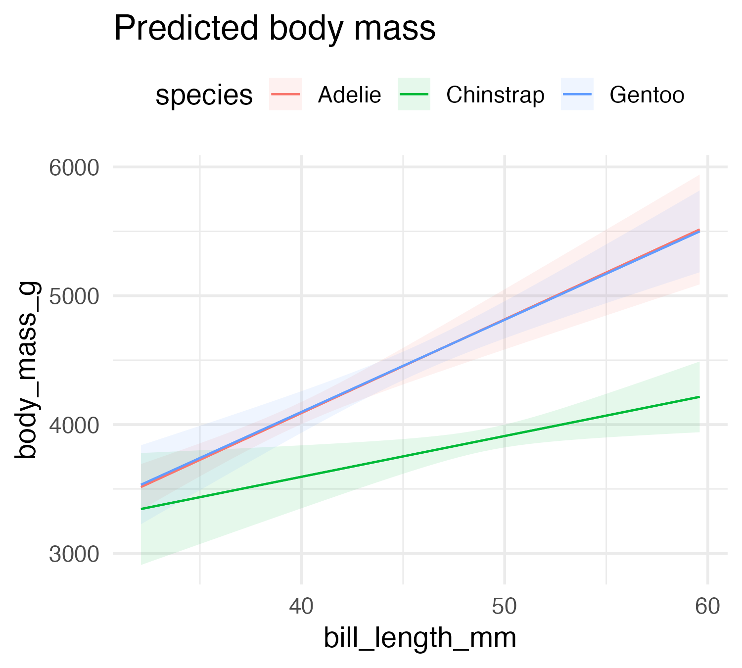
…others, not so much
| Characteristic | Beta | 95% CI1 | p-value |
|---|---|---|---|
| bill_length_mm | 73 | 52, 94 | <0.001 |
| species | |||
| Adelie | — | — | |
| Chinstrap | 1,146 | -282, 2,575 | 0.12 |
| Gentoo | 55 | -1,165, 1,274 | >0.9 |
| flipper_length_mm | 27 | 21, 34 | <0.001 |
| bill_length_mm * species | |||
| bill_length_mm * Chinstrap | -41 | -73, -9.4 | 0.011 |
| bill_length_mm * Gentoo | -1.2 | -30, 27 | >0.9 |
| 1 CI = Confidence Interval | |||
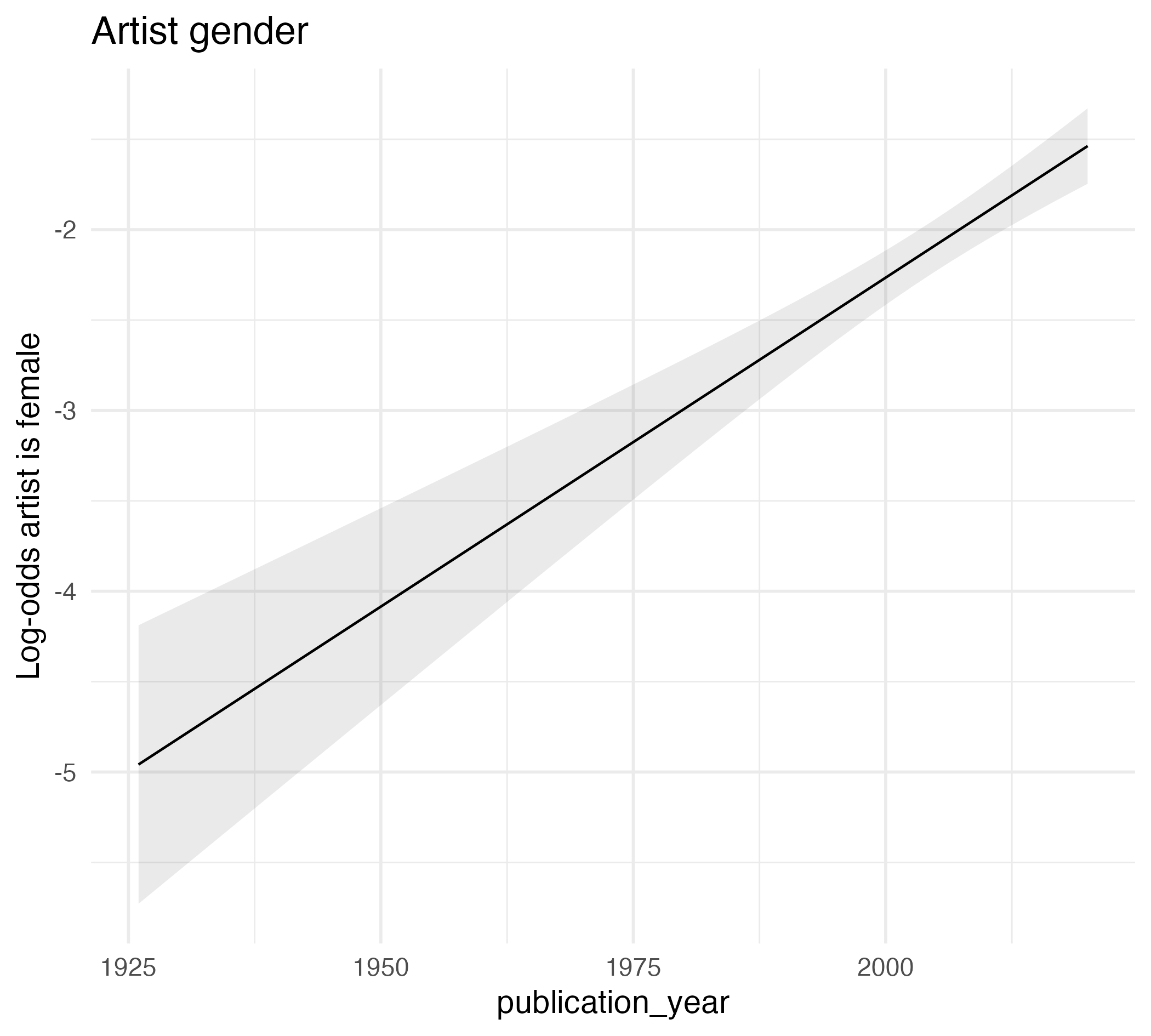
Art history
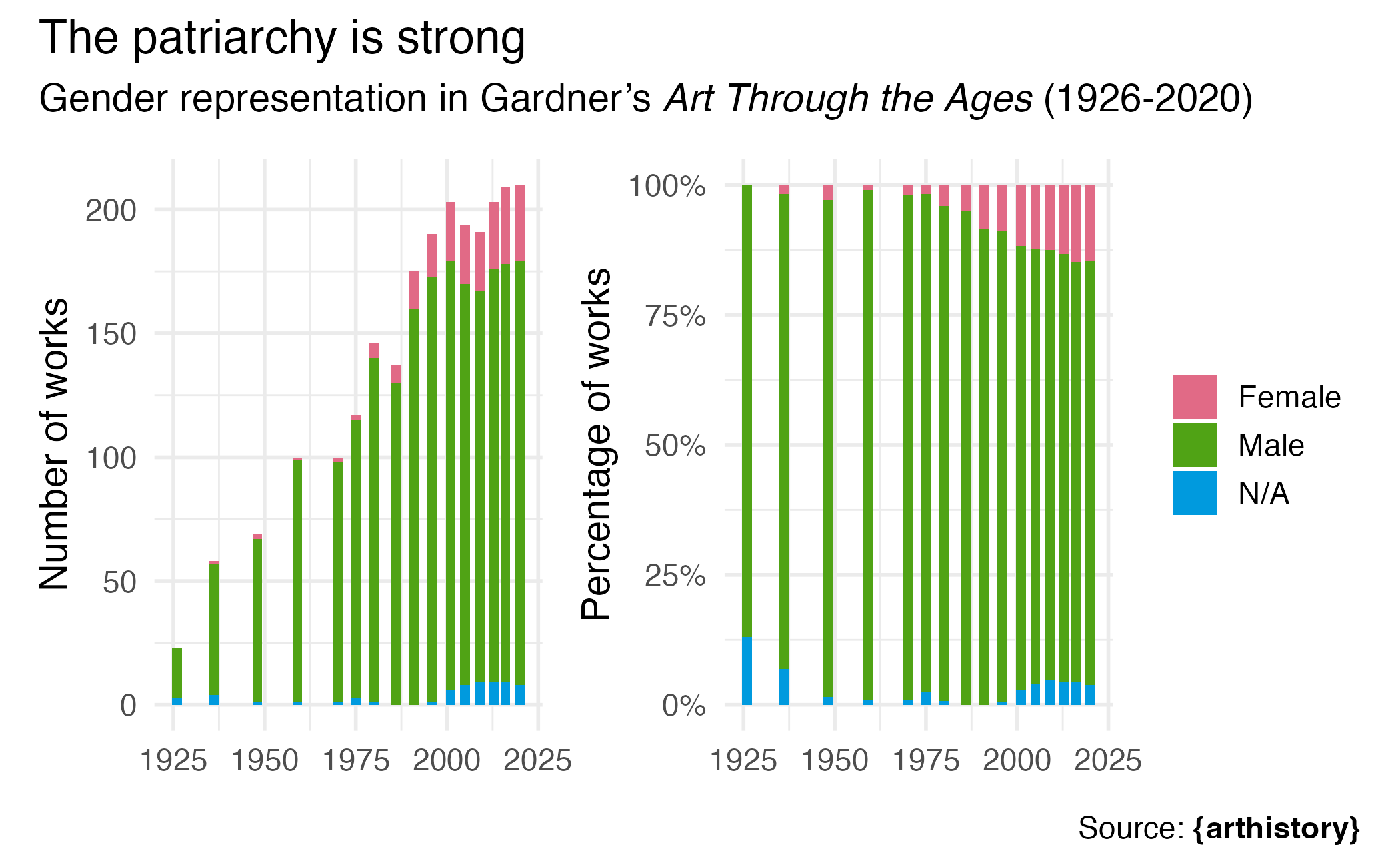
Gender representation in Gardner’s Art Through the Ages (1926-2020)
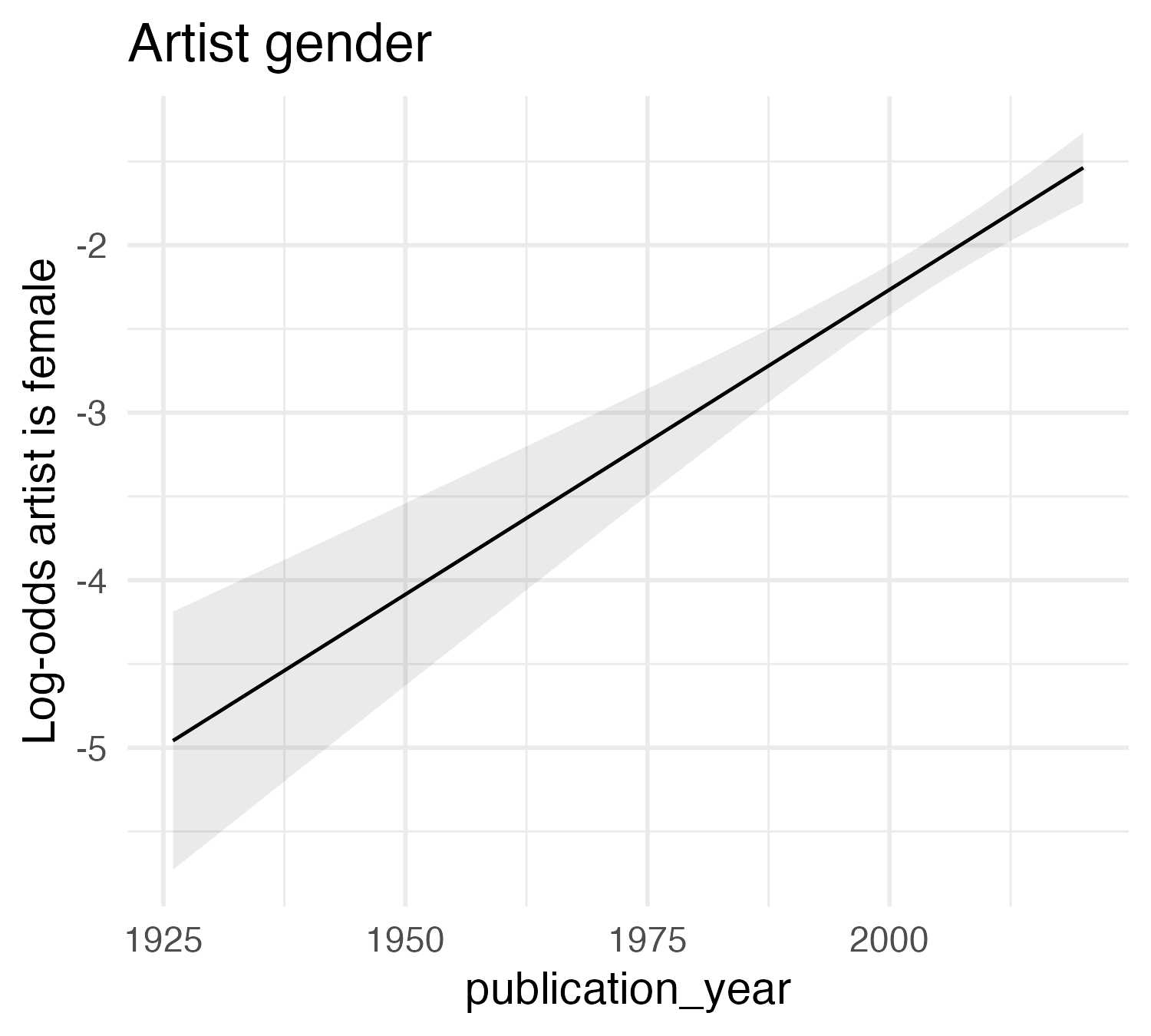
| Characteristic | log(OR)1 | 95% CI1 | p-value |
|---|---|---|---|
| publication_year | 0.04 | 0.03, 0.05 | <0.001 |
| 1 OR = Odds Ratio, CI = Confidence Interval | |||
Marginal effect of a non-linear slope
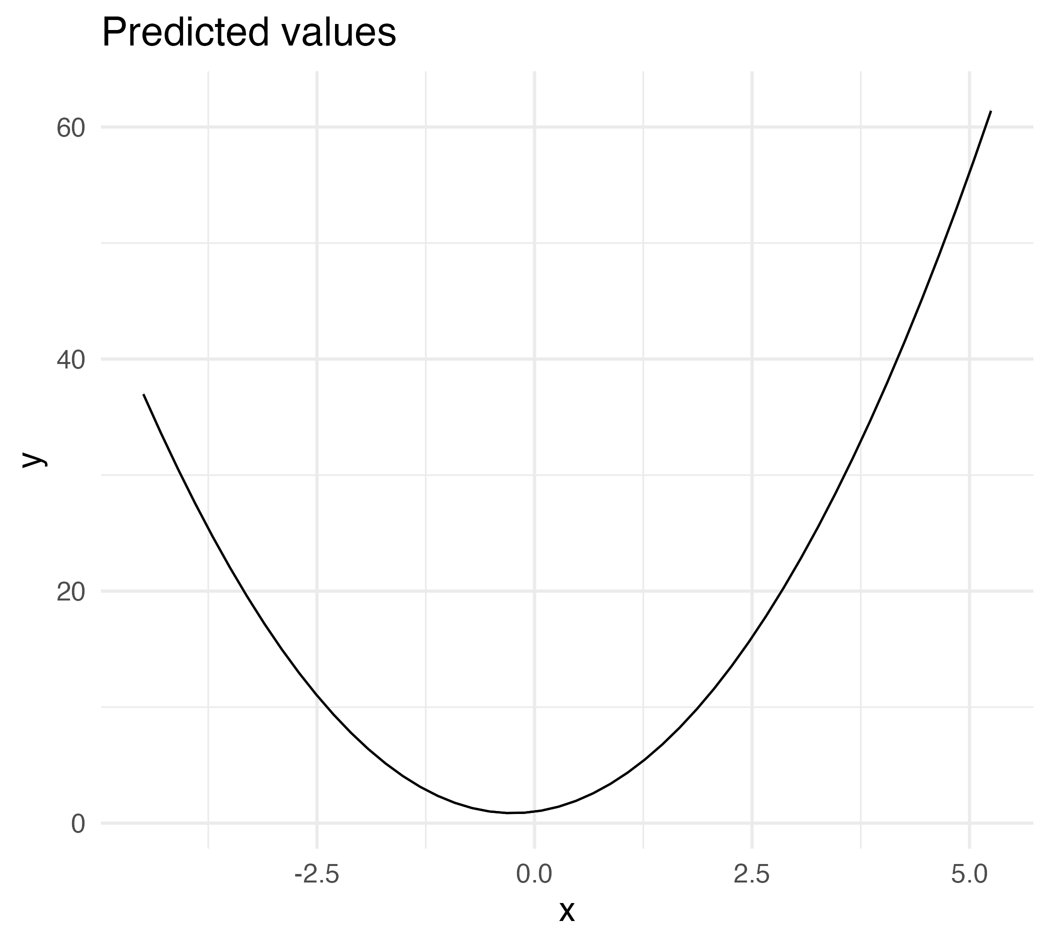
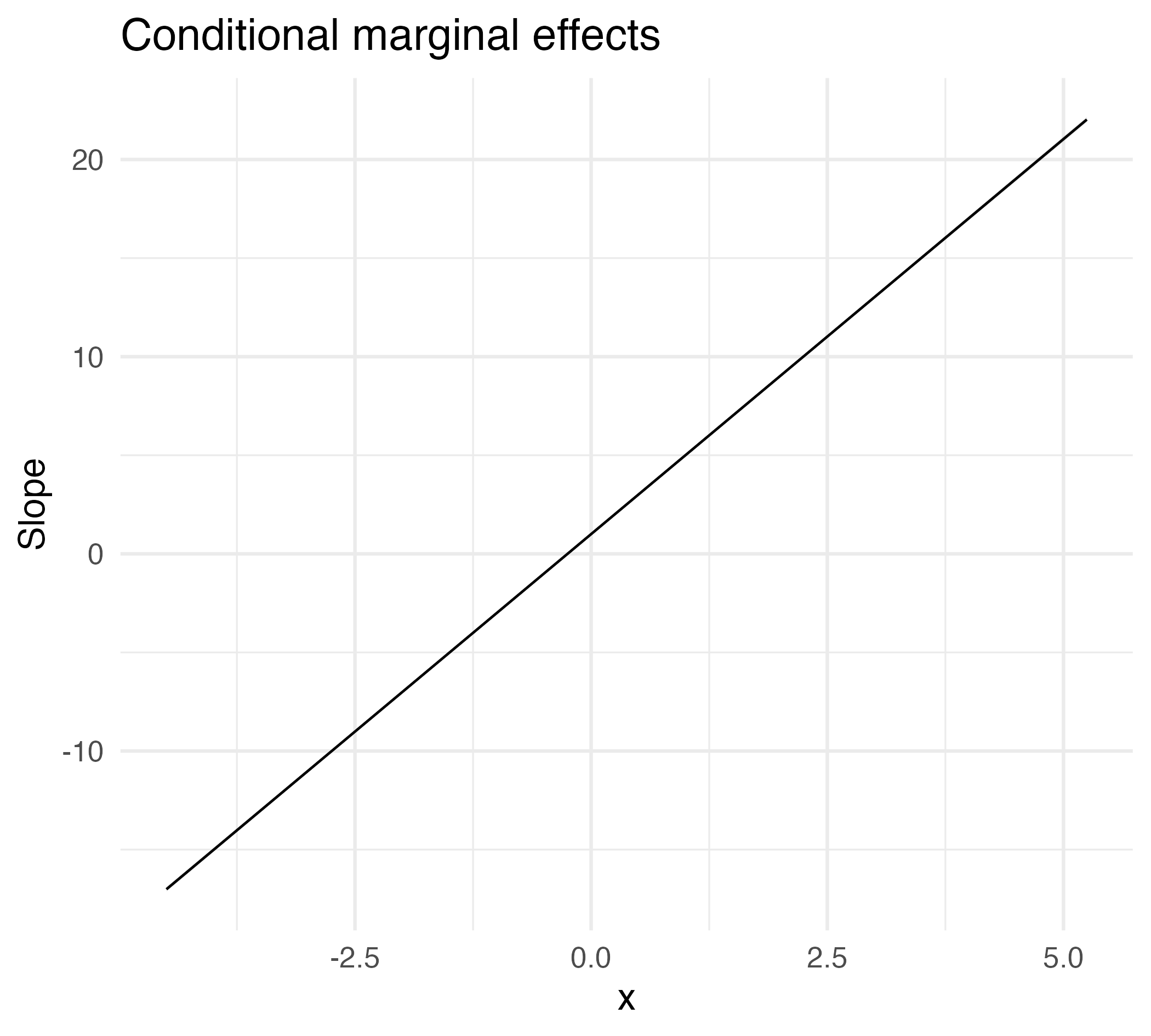
Marginal effect of a non-linear slope
Intepreting statistical models with marginaleffects
marginaleffects
marginaleffects is an R (and Python) package that provides a simple way to interpret results from a range of regression models
Implements a standardized interface for nearly 100 model types
Predictions
Predictions
- Estimate predictions from a model for specific values of the predictors
- What is the expected price for a three-bedroom house in a suburban area, adjusting for the house’s size, age, local amenities, and the current real estate market conditions?
- What is the expected turnout for elections in rural and urban areas, adjusting for national voting intentions and democratic characteristics?
- Estimate predictions from a model for average values in the dataset
- Average predicted outcome in the whole dataset
- Average predicted outcome for distinct subgroups in the data
- Emphasis on estimating predictions on the response scale
Predictions of penguin body mass
lm_mod <- linear_reg() |>
fit(body_mass_g ~ bill_length_mm + species, data = penguins) |>
extract_fit_engine()
pred <- predictions(lm_mod)
head(pred)- 1
- Extract the underlying fit object for marginaleffects
Estimate Std. Error z Pr(>|z|) S 2.5 % 97.5 %
3729 30.6 122 <0.001 Inf 3669 3789
3765 30.9 122 <0.001 Inf 3705 3826
3839 32.3 119 <0.001 Inf 3775 3902
3509 33.8 104 <0.001 Inf 3443 3576
3747 30.7 122 <0.001 Inf 3687 3807
3711 30.6 121 <0.001 Inf 3651 3770
Columns: rowid, estimate, std.error, statistic, p.value, s.value, conf.low, conf.high, body_mass_g, bill_length_mm, species
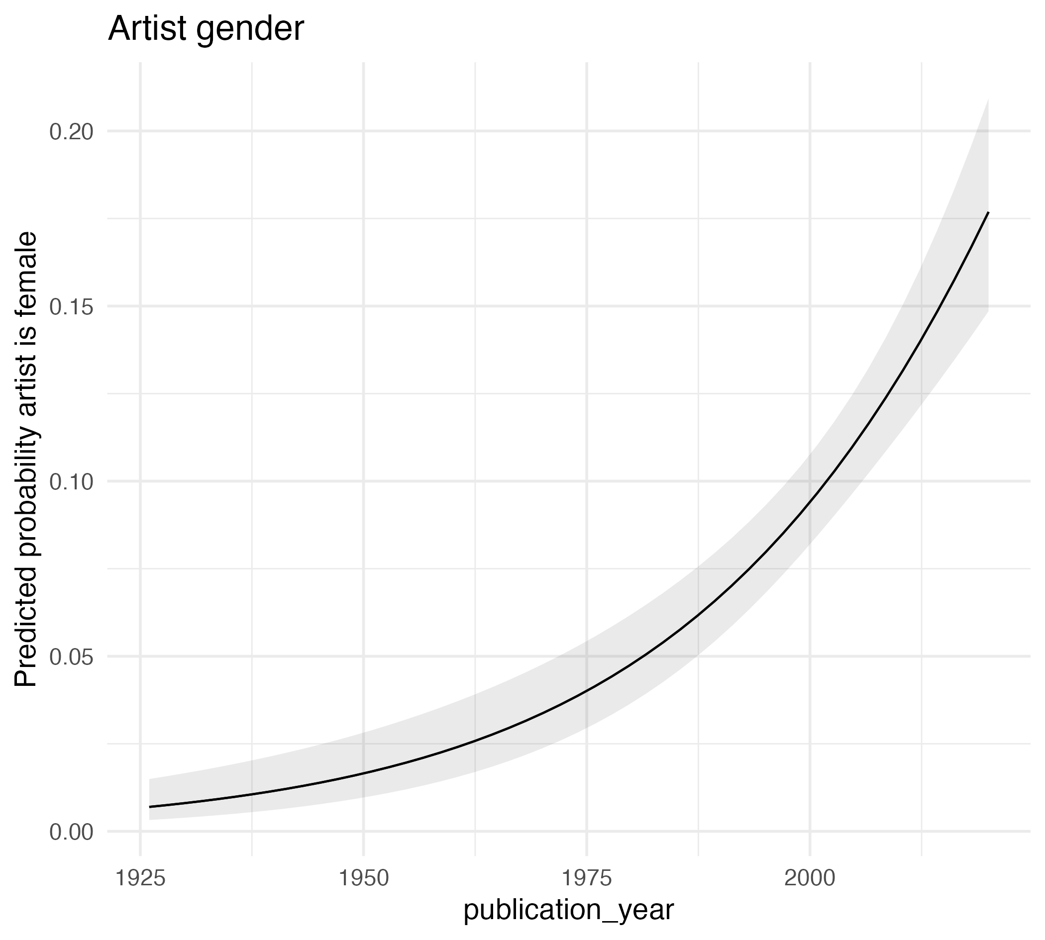
Type: response Predictions of artist gender
glm_mod <- logistic_reg() |>
  fit(artist_gender ~ publication_year, data = artist_subset) |>
  extract_fit_engine()

pred <- predictions(glm_mod, type = "response")
head(pred)
 Estimate Std. Error    z Pr(>|z|)     S  2.5 % 97.5 %
   0.0696    0.00640 10.9   <0.001  89.2 0.0571 0.0821
   0.0823    0.00638 12.9   <0.001 124.3 0.0698 0.0948
   0.0972    0.00662 14.7   <0.001 159.7 0.0842 0.1101
   0.1107    0.00725 15.3   <0.001 172.5 0.0965 0.1249
   0.1259    0.00847 14.9   <0.001 163.4 0.1093 0.1425
   0.1428    0.01040 13.7   <0.001 140.2 0.1224 0.1632

Columns: rowid, estimate, std.error, statistic, p.value, s.value, conf.low, conf.high, artist_gender, publication_year
Type:  response
 Estimate Std. Error     z Pr(>|z|)     S 2.5 % 97.5 %
    -2.59     0.0988 -26.2   <0.001 502.0 -2.79  -2.40
    -2.41     0.0844 -28.6   <0.001 594.1 -2.58  -2.25
    -2.23     0.0754 -29.5   <0.001 634.9 -2.38  -2.08
    -2.08     0.0736 -28.3   <0.001 582.6 -2.23  -1.94
    -1.94     0.0770 -25.2   <0.001 461.8 -2.09  -1.79
    -1.79     0.0849 -21.1   <0.001 326.0 -1.96  -1.63

Columns: rowid, estimate, std.error, statistic, p.value, s.value, conf.low, conf.high, artist_gender, publication_year
Type:  link
Grid of profiles
- Profile - combination of values of the predictor variables
- Grid - collection of one or more profiles
- Profiles do not have to correspond to actual observations in the dataset
- All observations in the dataset
- Average values of each variable
- Specific observed (or hypothetical) values of the predictors
- Context-dependent - what do you (or your audience) want to know?
Empirical distribution
 Estimate Std. Error     z Pr(>|z|)   S 2.5 % 97.5 %
     3729       30.6 121.8   <0.001 Inf  3669   3789
     3765       30.9 121.7   <0.001 Inf  3705   3826
     3839       32.3 119.0   <0.001 Inf  3775   3902
     3509       33.8 103.9   <0.001 Inf  3443   3576
     3747       30.7 121.9   <0.001 Inf  3687   3807
--- 332 rows omitted. See ?avg_predictions and ?print.marginaleffects ---
     4370       66.1  66.1   <0.001 Inf  4240   4500
     3245       58.5  55.5   <0.001 Inf  3131   3360
     3803       45.8  83.0   <0.001 Inf  3713   3893
     3913       47.5  82.4   <0.001 Inf  3820   4006
     3858       46.5  83.0   <0.001 Inf  3767   3949
Columns: rowid, estimate, std.error, statistic, p.value, s.value, conf.low, conf.high, body_mass_g, bill_length_mm, species
Type:  response
User-specified values
Hypothetical values
predictions(lm_mod, newdata = datagrid(
  species = "Adelie",
  bill_length_mm = c(30, 40, 50, 60),
  model = lm_mod
))
 species bill_length_mm Estimate Std. Error     z Pr(>|z|)   S 2.5 % 97.5 %
  Adelie             30     2897       67.8  42.7   <0.001 Inf  2764   3030
  Adelie             40     3811       31.7 120.4   <0.001 Inf  3749   3873
  Adelie             50     4726       83.0  56.9   <0.001 Inf  4563   4888
  Adelie             60     5640      149.2  37.8   <0.001 Inf  5347   5932

Columns: rowid, estimate, std.error, statistic, p.value, s.value, conf.low, conf.high, species, bill_length_mm, body_mass_g
Type:  response
User-specified values
Average values
predictions(lm_mod, newdata = datagrid(
  FUN_factor = unique, FUN_numeric = median, model = lm_mod
))
 Estimate Std. Error     z Pr(>|z|)   S 2.5 % 97.5 % bill_length_mm   species
     4218       49.5  85.2   <0.001 Inf  4121   4315           44.5 Adelie
     4797       39.8 120.4   <0.001 Inf  4719   4875           44.5 Gentoo
     3332       54.6  61.0   <0.001 Inf  3225   3439           44.5 Chinstrap

Columns: rowid, estimate, std.error, statistic, p.value, s.value, conf.low, conf.high, bill_length_mm, species, body_mass_g
Type:  response
Representative values
Adjusted prediction at the mean - predicted outcome when all regressors are held at their mean (or mode)
Aggregating predictions
- Hard to communicate results if number of observations is large
- Compute aggregated predictions for the entire dataset, or distinct subgroups
Average predictions
gender_year_national_fit <- logistic_reg() |>
  fit(artist_gender ~ publication_year * artist_nationality, data = artist_subset) |>
  extract_fit_engine()

avg_predictions(gender_year_national_fit)
Estimate Pr(>|z|) S 2.5 % 97.5 %
0.066 <0.001 443.2 0.0541 0.0802
Columns: estimate, p.value, s.value, conf.low, conf.high
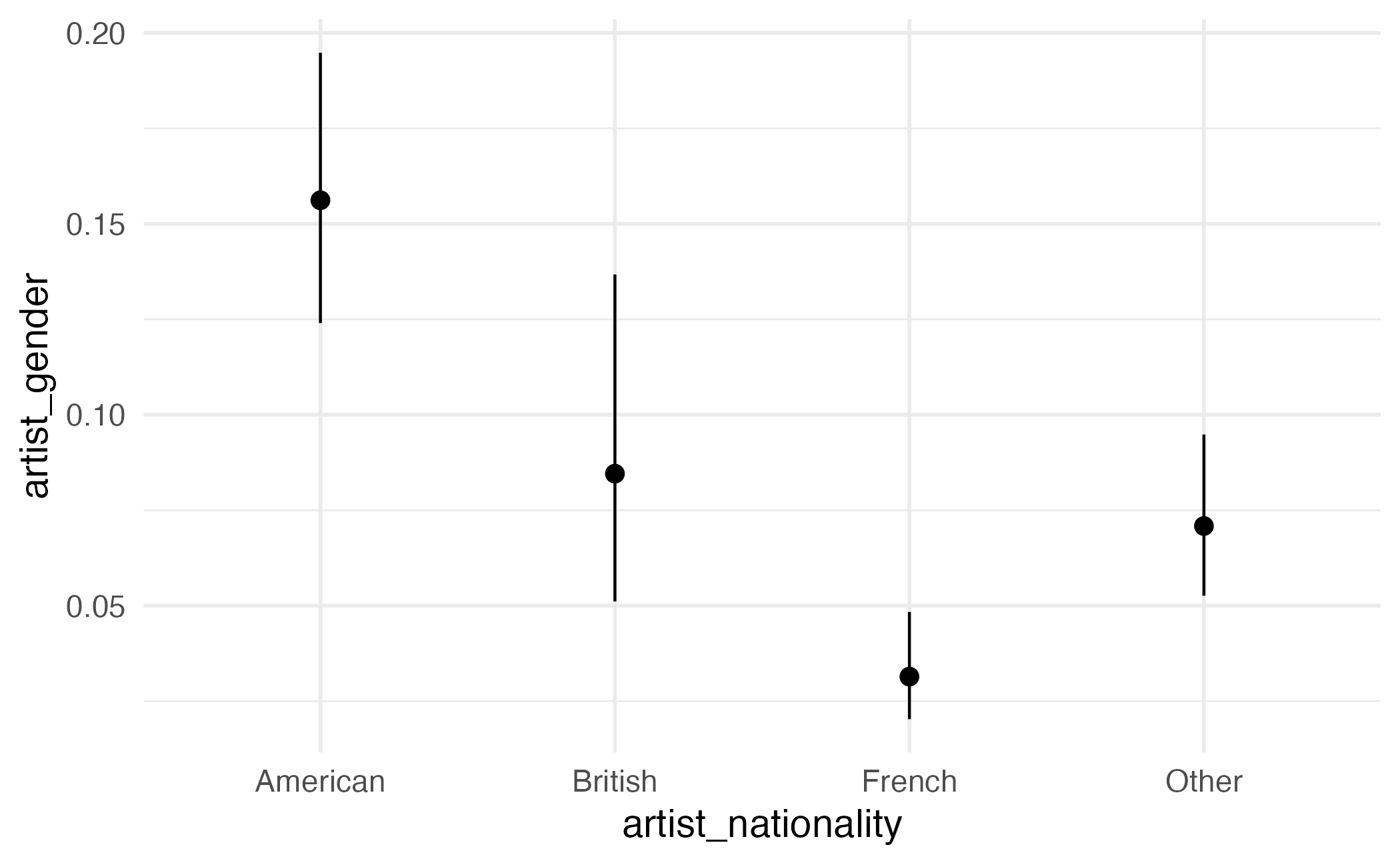
Type: invlink(link) Average predictions by group
 artist_nationality Estimate Pr(>|z|)     S  2.5 % 97.5 %
           American   0.1661   <0.001 118.9 0.1342 0.2038
           French     0.0289   <0.001 152.2 0.0181 0.0459
           Other      0.0729   <0.001 192.2 0.0546 0.0968
           British    0.0820   <0.001  55.9 0.0488 0.1346

Columns: artist_nationality, estimate, p.value, s.value, conf.low, conf.high
Type:  invlink(link)
Visualizing predictions
Visualizing predictions
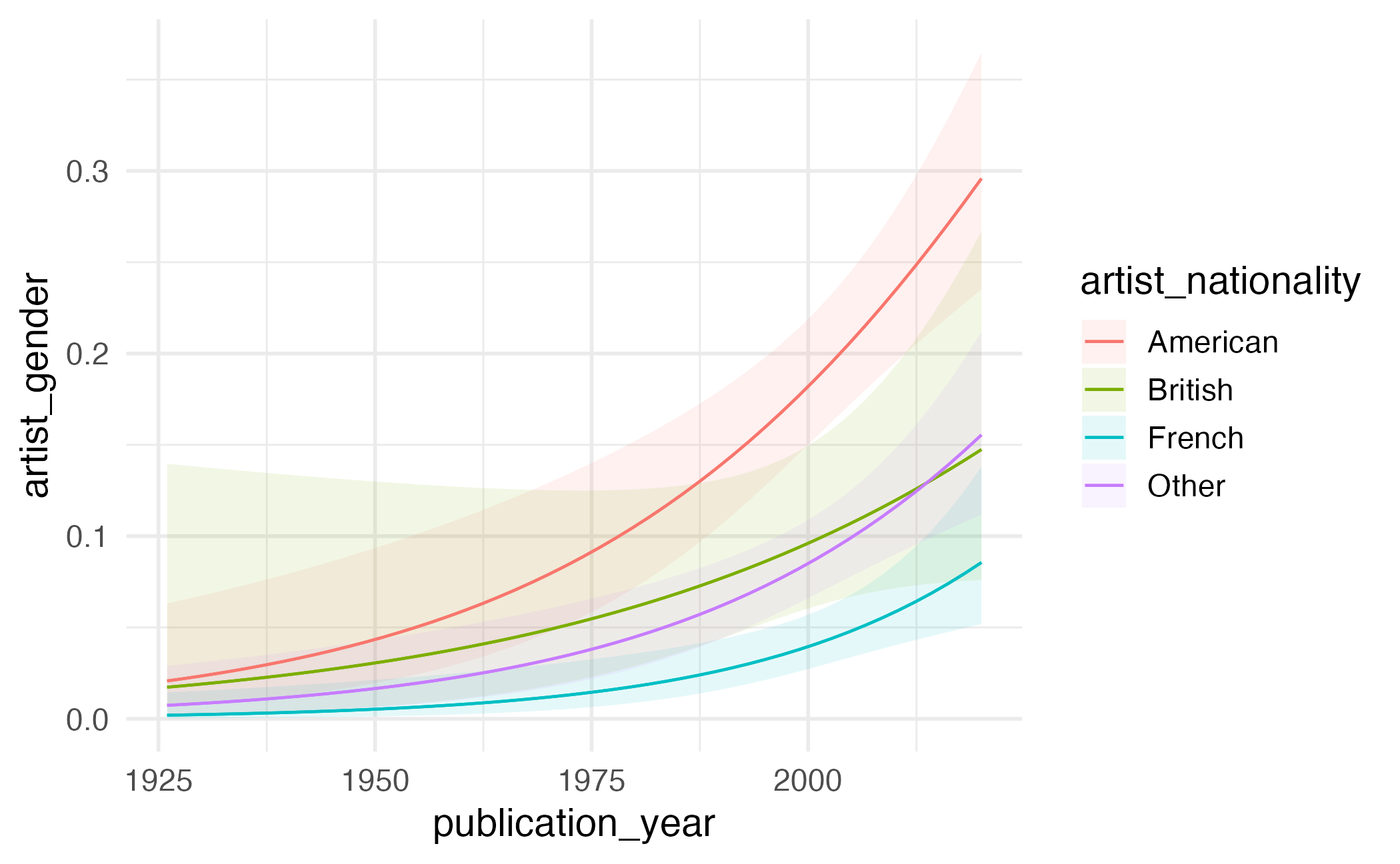
Customizing plots
plot_predictions(gender_year_national_fit,
  condition = c("publication_year", "artist_nationality")
) +
scale_y_continuous(labels = label_percent()) +
scale_color_OkabeIto(aesthetics = c("color", "fill"), guide = "none") +
facet_wrap(facets = vars(artist_nationality)) +
labs(
x = "Publication year",
y = "Predicted probability artist is female"
) +
theme(legend.position = "top")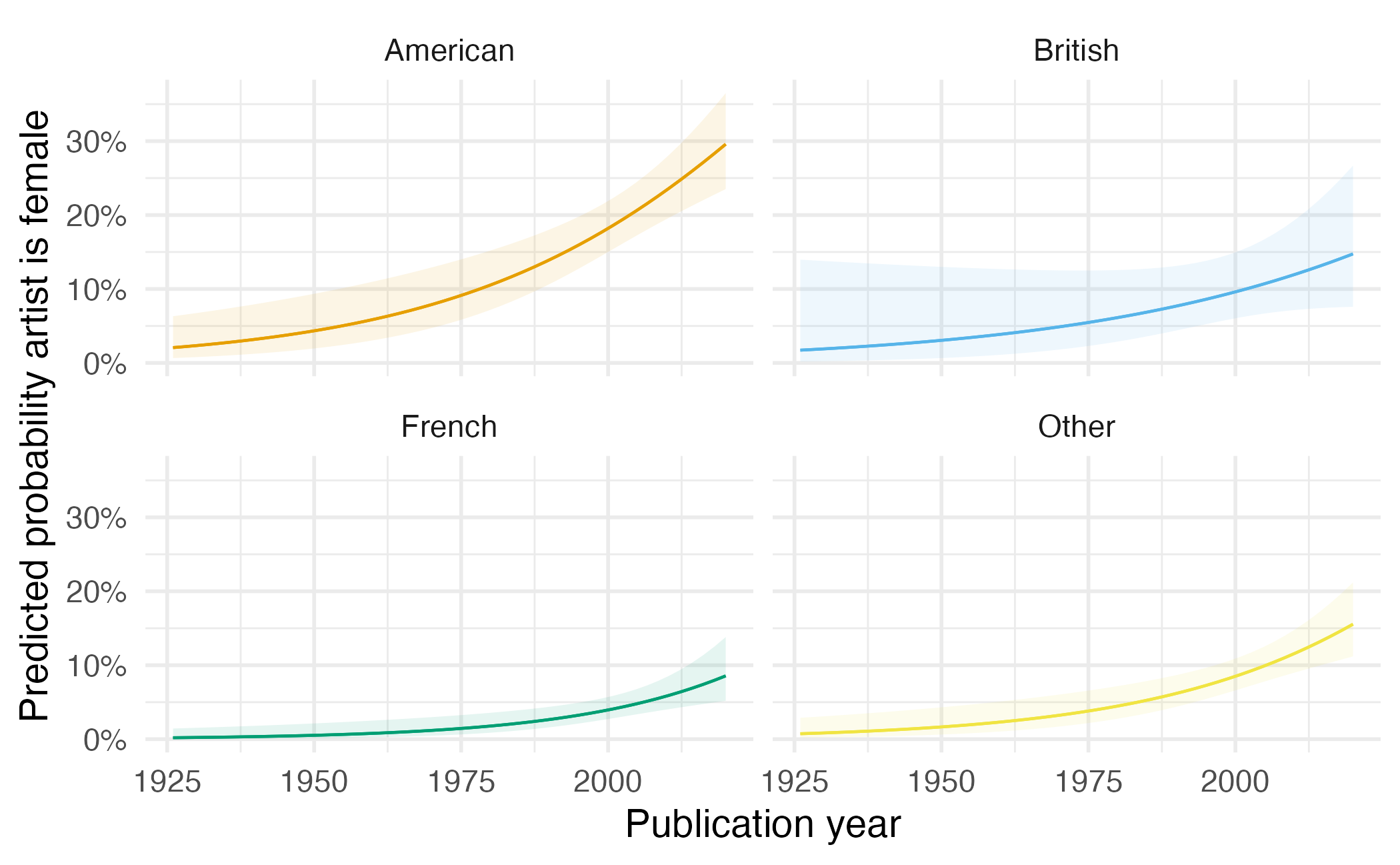
Comparisons
Comparisons
Functions of two or more predictions
- Differences
- Risk ratios
- Relative odds
Comparisons are useful for
- Understanding the relationship between predictors and the outcome
- Comparing the effect of different predictors
- Communicating results to a non-technical audience
Quantity of interest
- Predictor type - how does the explanator of interest change?
- Numeric variable - one-unit increase
- Categorical variable - difference between one category and its baseline
- Comparison type - how do we compare the two predicted outcomes?
- Difference - how much does the outcome change?
- Ratio - how many times does the outcome change?
- Odds - how many times more likely is the outcome?
Differences
# hypothetical artist
artist <- tibble(
  publication_year = 1950,
  artist_nationality = "American"
)

comparisons(gender_year_national_fit, newdata = artist)
               Term           Contrast Estimate Std. Error     z Pr(>|z|)    S
 artist_nationality British - American -0.01286   0.029251 -0.44    0.660  0.6
 artist_nationality French - American  -0.03818   0.017803 -2.14    0.032  5.0
 artist_nationality Other - American   -0.02687   0.019224 -1.40    0.162  2.6
 publication_year   +1                  0.00134   0.000225  5.96   <0.001 28.6
     2.5 %   97.5 % publication_year artist_nationality
 -0.070190  0.04447             1950           American
 -0.073077 -0.00329             1950           American
 -0.064543  0.01081             1950           American
  0.000899  0.00178             1950           American

Columns: rowid, term, contrast, estimate, std.error, statistic, p.value, s.value, conf.low, conf.high, predicted_lo, predicted_hi, predicted, publication_year, artist_nationality, artist_gender
Type:  response
Differences
               Term           Contrast Estimate Std. Error      z Pr(>|z|)   S
 artist_nationality British / American    0.704    0.61052   1.15    0.249 2.0
 artist_nationality French / American     0.121    0.09944   1.21    0.225 2.2
 artist_nationality Other / American      0.381    0.24246   1.57    0.116 3.1
 publication_year   +1                    1.031    0.00782 131.84   <0.001 Inf
   2.5 % 97.5 % publication_year artist_nationality
 -0.4927  1.901             1950           American
 -0.0742  0.316             1950           American
 -0.0939  0.857             1950           American
  1.0155  1.046             1950           American

Columns: rowid, term, contrast, estimate, std.error, statistic, p.value, s.value, conf.low, conf.high, predicted_lo, predicted_hi, predicted, publication_year, artist_nationality, artist_gender
Type:  response
Differences
             Term Contrast Estimate Std. Error    z Pr(>|z|)    S  2.5 % 97.5 %
 publication_year      +10   0.0153    0.00213 7.18   <0.001 40.4 0.0111 0.0195
 publication_year artist_nationality
             1950           American

Columns: rowid, term, contrast, estimate, std.error, statistic, p.value, s.value, conf.low, conf.high, predicted_lo, predicted_hi, predicted, publication_year, artist_nationality, artist_gender
Type:  response
Conditional differences
In most models, the effect of a predictor depends on the values of other predictors
- Linear regression (with interaction terms, quadratic terms, etc.)
- Logistic regression
- Poisson regression
- Survival models
What comparisons do we want to make? What portion of the predictor space do we cover?
- Empirical distribution
- User-specified values
- Representative values
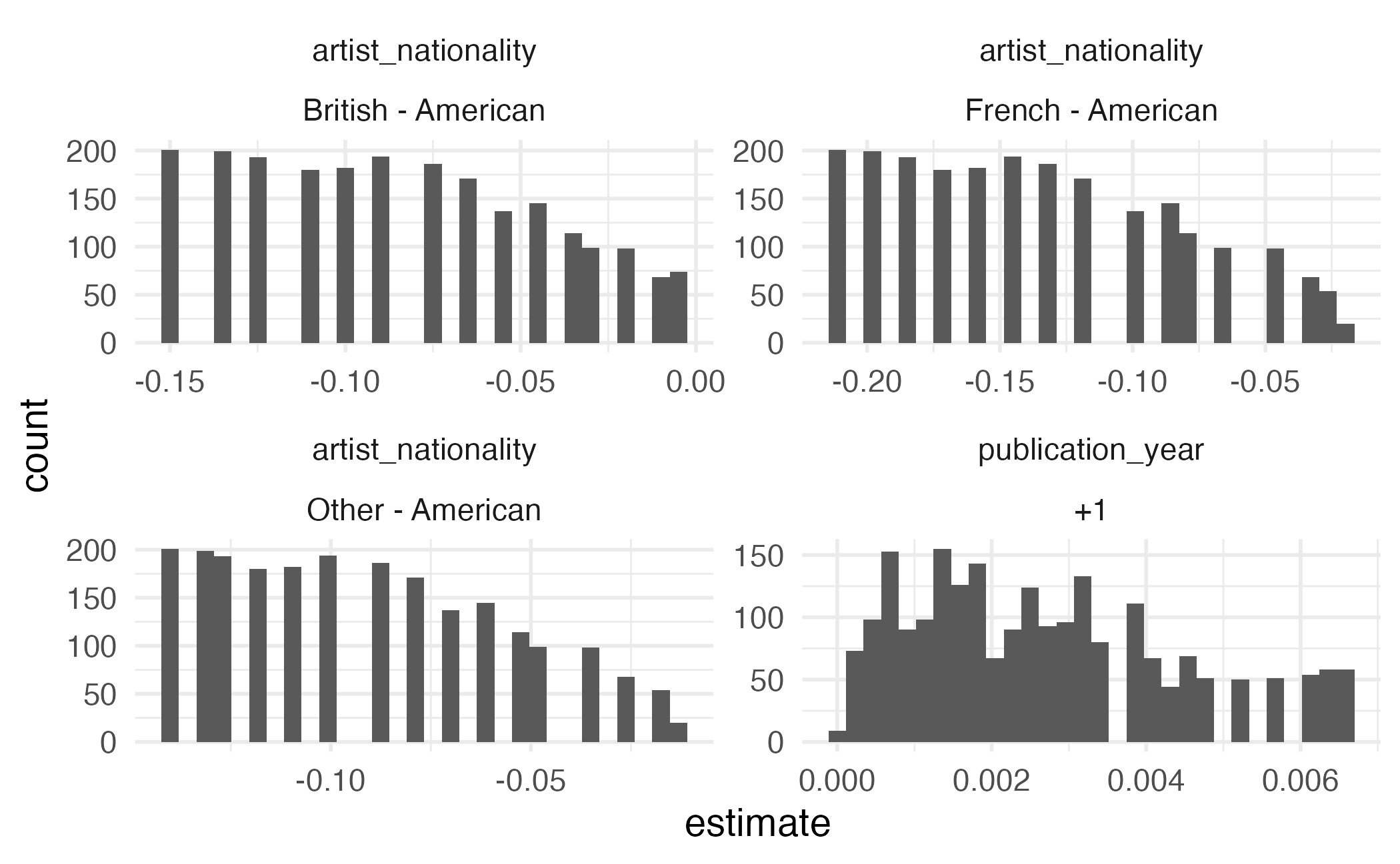
Empirical distribution
             Term Contrast Estimate Std. Error    z Pr(>|z|)    S   2.5 %
 publication_year       +1  0.00394   0.000716 5.51  < 0.001 24.8 0.00254
 publication_year       +1  0.00440   0.000906 4.86  < 0.001 19.7 0.00263
 publication_year       +1  0.00488   0.001113 4.38  < 0.001 16.4 0.00269
 publication_year       +1  0.00526   0.001286 4.09  < 0.001 14.5 0.00274
 publication_year       +1  0.00565   0.001459 3.87  < 0.001 13.2 0.00279
  97.5 %
 0.00535
 0.00618
 0.00706
 0.00778
 0.00851
--- 2231 rows omitted. See ?avg_comparisons and ?print.marginaleffects ---
 publication_year       +1  0.00383   0.001285 2.98  0.00292 8.4 0.00131
 publication_year       +1  0.00412   0.001450 2.84  0.00446 7.8 0.00128
 publication_year       +1  0.00454   0.001681 2.70  0.00693 7.2 0.00124
 publication_year       +1  0.00412   0.001450 2.84  0.00446 7.8 0.00128
 publication_year       +1  0.00454   0.001681 2.70  0.00693 7.2 0.00124
  97.5 %
 0.00635
 0.00697
 0.00783
 0.00697
 0.00783
Columns: rowid, term, contrast, estimate, std.error, statistic, p.value, s.value, conf.low, conf.high, predicted_lo, predicted_hi, predicted, artist_gender, publication_year, artist_nationality
Type:  response
               Term           Contrast Estimate Std. Error     z Pr(>|z|)   S
 artist_nationality British - American -0.06448    0.02837 -2.27  0.02302 5.4
 artist_nationality British - American -0.07582    0.02782 -2.73  0.00642 7.3
 artist_nationality British - American -0.08852    0.02875 -3.08  0.00207 8.9
 artist_nationality British - American -0.09964    0.03124 -3.19  0.00143 9.5
 artist_nationality British - American -0.11161    0.03570 -3.13  0.00177 9.1
    2.5 %   97.5 %
 -0.12007 -0.00888
 -0.13035 -0.02130
 -0.14486 -0.03218
 -0.16088 -0.03840
 -0.18158 -0.04164
--- 8954 rows omitted. See ?avg_comparisons and ?print.marginaleffects ---
 publication_year   +1                  0.00383    0.00129  2.98  0.00292 8.4
 publication_year   +1                  0.00412    0.00145  2.84  0.00446 7.8
 publication_year   +1                  0.00454    0.00168  2.70  0.00693 7.2
 publication_year   +1                  0.00412    0.00145  2.84  0.00446 7.8
 publication_year   +1                  0.00454    0.00168  2.70  0.00693 7.2
    2.5 %   97.5 %
  0.00131  0.00635
  0.00128  0.00697
  0.00124  0.00783
  0.00128  0.00697
  0.00124  0.00783
Columns: rowid, term, contrast, estimate, std.error, statistic, p.value, s.value, conf.low, conf.high, predicted_lo, predicted_hi, predicted, artist_gender, publication_year, artist_nationality
Type:  response
Empirical distribution
User-specified values
# French artist in 1950
comparisons(
  gender_year_national_fit,
  newdata = datagrid(
    publication_year = 1950,
    artist_nationality = "French"
  )
)
               Term           Contrast publication_year artist_nationality
 artist_nationality British - American             1950             French
 artist_nationality French - American              1950             French
 artist_nationality Other - American               1950             French
 publication_year   +1                             1950             French
  Estimate Std. Error     z Pr(>|z|)   S     2.5 %    97.5 %
 -0.012858   2.93e-02 -0.44   0.6602 0.6 -7.02e-02  0.044474
 -0.038184   1.78e-02 -2.14   0.0320 5.0 -7.31e-02 -0.003291
 -0.026865   1.92e-02 -1.40   0.1623 2.6 -6.45e-02  0.010813
  0.000219   9.11e-05  2.40   0.0163 5.9  4.03e-05  0.000397

Columns: rowid, term, contrast, estimate, std.error, statistic, p.value, s.value, conf.low, conf.high, publication_year, artist_nationality, predicted_lo, predicted_hi, predicted, artist_gender
Type:  response
Representative values
               Term           Contrast Estimate Std. Error     z Pr(>|z|)    S
 artist_nationality British - American -0.07161   0.027900 -2.57   0.0103  6.6
 artist_nationality French - American  -0.12476   0.019320 -6.46   <0.001 33.1
 artist_nationality Other - American   -0.08531   0.020937 -4.07   <0.001 14.4
 publication_year   +1                  0.00128   0.000335  3.80   <0.001 12.8
     2.5 %   97.5 % publication_year artist_nationality
 -0.126292 -0.01693             1994             French
 -0.162627 -0.08689             1994             French
 -0.126349 -0.04428             1994             French
  0.000618  0.00193             1994             French

Columns: rowid, term, contrast, estimate, std.error, statistic, p.value, s.value, conf.low, conf.high, predicted_lo, predicted_hi, predicted, publication_year, artist_nationality, artist_gender
Type:  response
Warning
Computationally efficient, but only makes sense if the “average” individual actually exists in the dataset.
Aggregating comparisons
Same as with predictions
- Average comparison for the whole dataset
- Average comparison for distinct subgroups in the data
Average comparisons
               Term                       Contrast Estimate Std. Error     z
 artist_nationality mean(British) - mean(American) -0.08264   0.026459 -3.12
 artist_nationality mean(French) - mean(American)  -0.13410   0.017412 -7.70
 artist_nationality mean(Other) - mean(American)   -0.09095   0.018761 -4.85
 publication_year   mean(+1)                        0.00268   0.000409  6.55
 Pr(>|z|)    S    2.5 %   97.5 %
  0.00179  9.1 -0.13450 -0.03078
  < 0.001 46.1 -0.16823 -0.09997
  < 0.001 19.6 -0.12772 -0.05417
  < 0.001 34.0  0.00188  0.00348

Columns: term, contrast, estimate, std.error, statistic, p.value, s.value, conf.low, conf.high, predicted_lo, predicted_hi, predicted
Type:  response
Subgroups
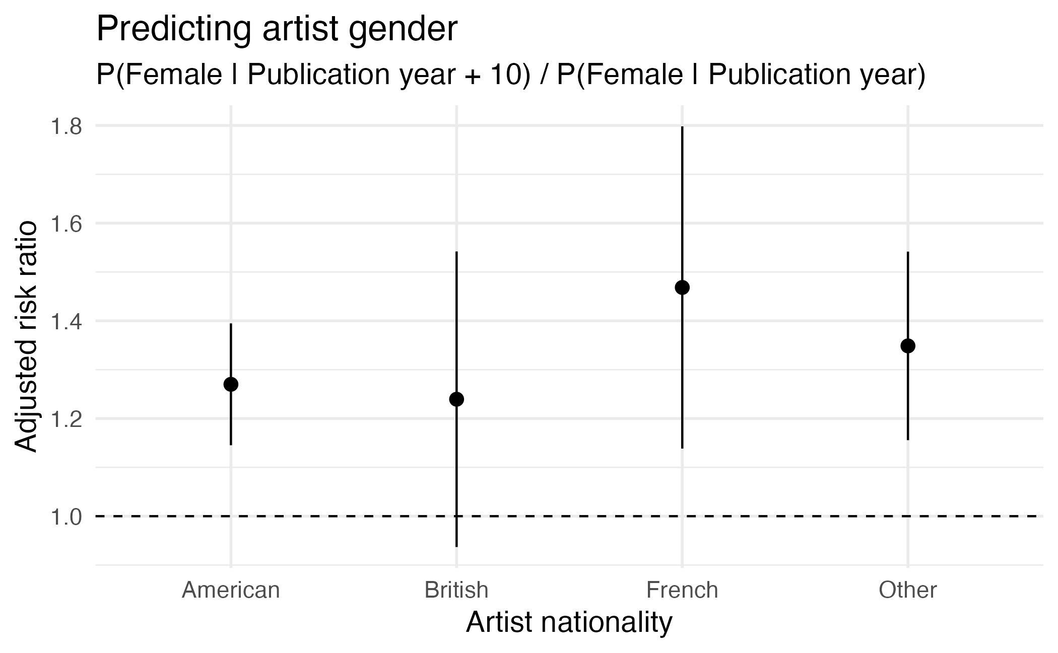
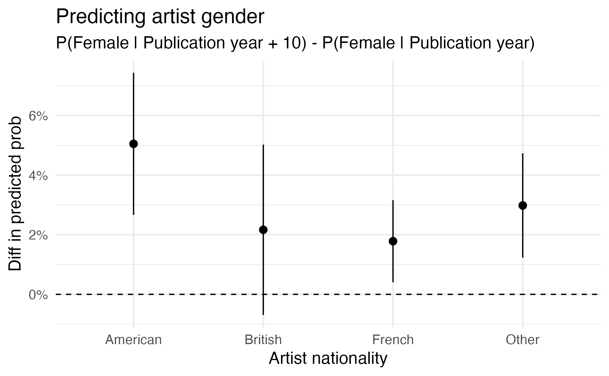
avg_comparisons(gender_year_national_fit,
  variables = list(publication_year = 10),
  by = "artist_nationality"
)
             Term  Contrast artist_nationality Estimate Std. Error    z
 publication_year mean(+10)           American   0.0505    0.01217 4.15
 publication_year mean(+10)           British    0.0217    0.01458 1.49
 publication_year mean(+10)           French     0.0178    0.00703 2.54
 publication_year mean(+10)           Other      0.0298    0.00893 3.34
 Pr(>|z|)    S    2.5 % 97.5 %
   <0.001 14.9  0.02666 0.0743
   0.1375  2.9 -0.00692 0.0502
   0.0112  6.5  0.00405 0.0316
   <0.001 10.2  0.01232 0.0473

Columns: term, contrast, artist_nationality, estimate, std.error, statistic, p.value, s.value, conf.low, conf.high, predicted_lo, predicted_hi, predicted
Type:  response
Visualizing comparisons
Visualizing comparisons
Slopes
Motivation
Partial derivatives of the regression equation with respect to a regressor of interest.1
- Marginal effects
- Trends
- Velocity
Since slopes are conditional quantities, they can be aggregated in a number of ways.
Average marginal effects

Average Marginal Effects (AME)
Term Contrast Estimate Std. Error z
bill_length_mm mean(dY/dX) 64.11 7.12 9.0034
flipper_length_mm mean(dY/dX) 27.26 3.18 8.5865
species mean(Chinstrap) - mean(Adelie) -656.05 94.90 -6.9128
species mean(Gentoo) - mean(Adelie) 3.65 95.21 0.0383
Pr(>|z|) S 2.5 % 97.5 %
<0.001 62.0 50.2 78.1
<0.001 56.6 21.0 33.5
<0.001 37.6 -842.1 -470.0
0.969 0.0 -183.0 190.3
Columns: term, contrast, estimate, std.error, statistic, p.value, s.value, conf.low, conf.high, predicted_lo, predicted_hi, predicted
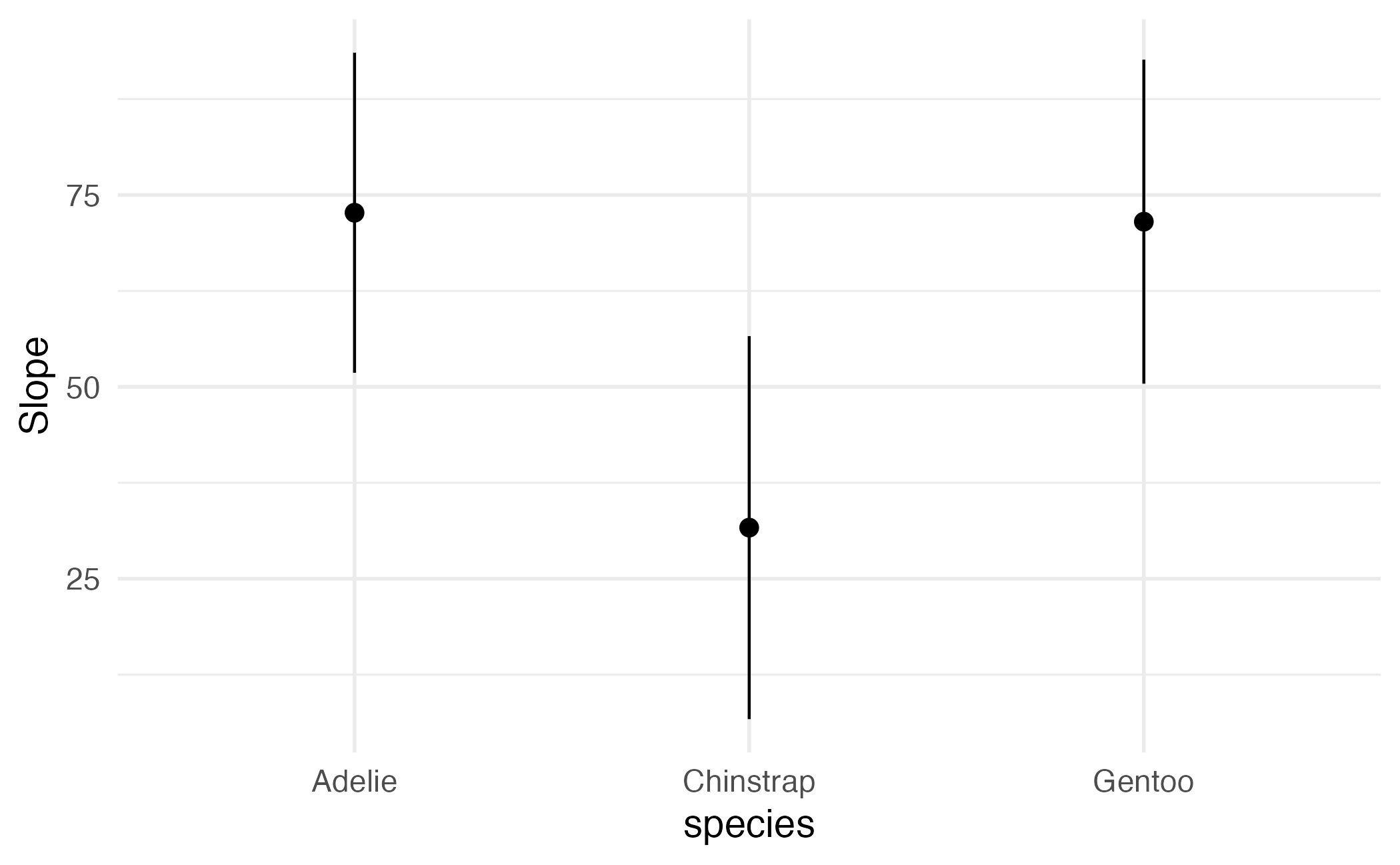
Type: response Group-Average Marginal Effects (G-AME)
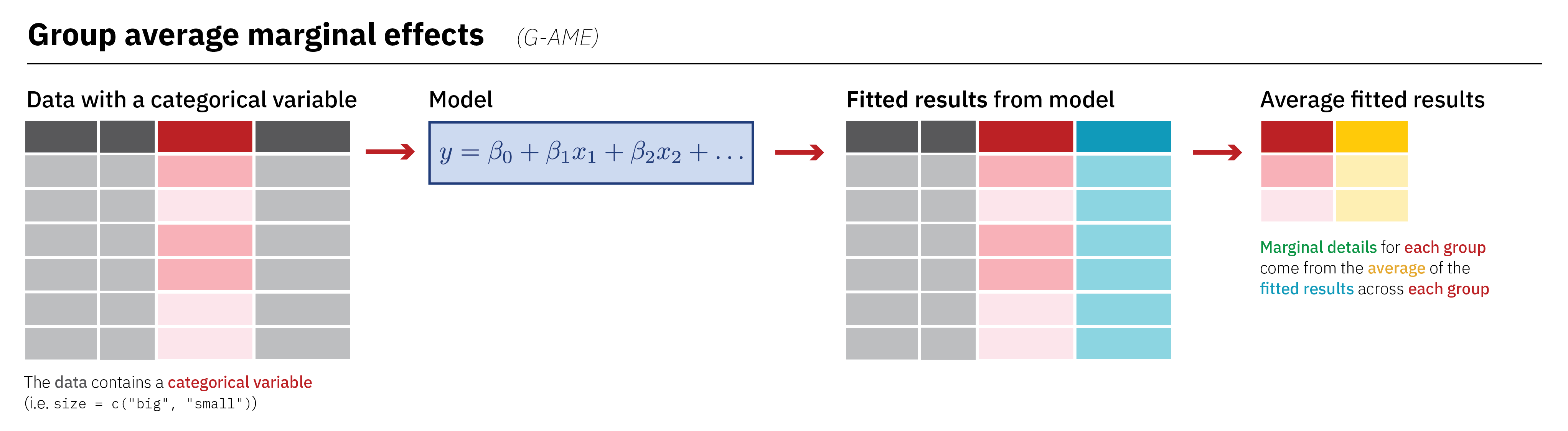
Group-Average Marginal Effects (G-AME)
           Term    Contrast   species Estimate Std. Error    z Pr(>|z|)    S
 bill_length_mm mean(dY/dX) Adelie        72.7       10.6 6.83   <0.001 36.8
 bill_length_mm mean(dY/dX) Chinstrap     31.7       12.7 2.48    0.013  6.3
 bill_length_mm mean(dY/dX) Gentoo        71.5       10.8 6.60   <0.001 34.5
 2.5 % 97.5 %
 51.83   93.5
  6.68   56.6
 50.28   92.8

Columns: term, contrast, species, estimate, std.error, statistic, p.value, s.value, conf.low, conf.high, predicted_lo, predicted_hi, predicted
Type:  response
Group-Average Marginal Effects (G-AME)
Group-Average Marginal Effects (G-AME)
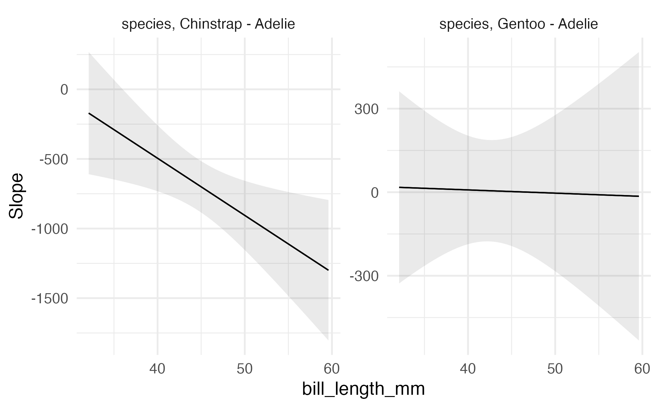
Marginal Effects at user-specified or Representative values (MER)
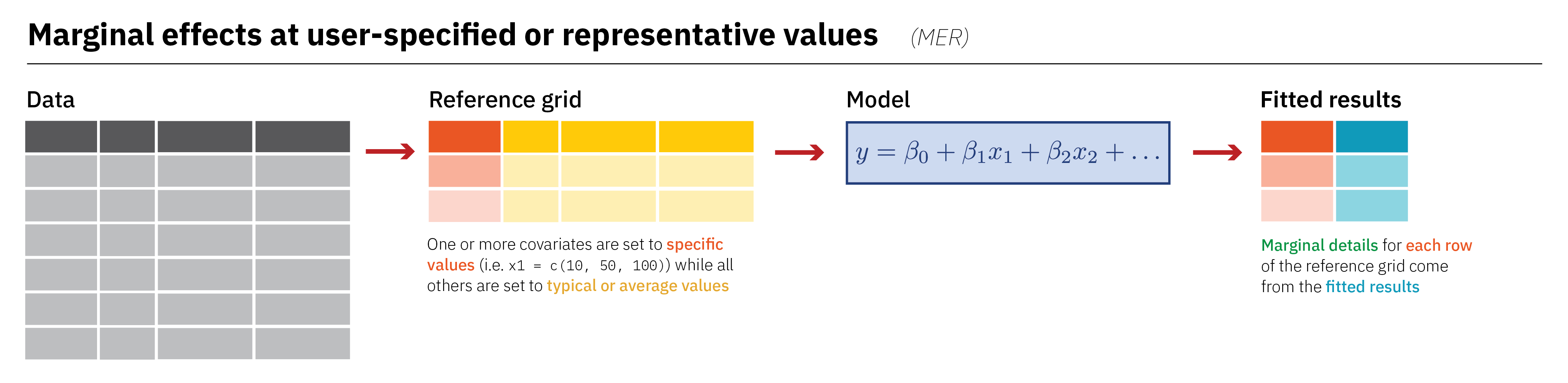
Marginal Effects at user-specified or Representative values (MER)
              Term           Contrast flipper_length_mm species Estimate
 bill_length_mm    dY/dX                            180  Adelie    72.69
 bill_length_mm    dY/dX                            180  Gentoo    71.53
 flipper_length_mm dY/dX                            180  Adelie    27.26
 flipper_length_mm dY/dX                            180  Gentoo    27.26
 species           Chinstrap - Adelie               180  Adelie  -656.05
 species           Chinstrap - Adelie               180  Gentoo  -656.05
 species           Gentoo - Adelie                  180  Adelie     3.65
 species           Gentoo - Adelie                  180  Gentoo     3.65
 Std. Error       z Pr(>|z|)    S  2.5 % 97.5 %
      10.64  6.8304   <0.001 36.8   51.8   93.6
      10.87  6.5830   <0.001 34.3   50.2   92.8
       3.17  8.5877   <0.001 56.6   21.0   33.5
       3.18  8.5844   <0.001 56.6   21.0   33.5
      94.90 -6.9128   <0.001 37.6 -842.1 -470.0
      94.90 -6.9128   <0.001 37.6 -842.1 -470.0
      95.21  0.0383    0.969  0.0 -183.0  190.3
      95.21  0.0383    0.969  0.0 -183.0  190.3

Columns: rowid, term, contrast, estimate, std.error, statistic, p.value, s.value, conf.low, conf.high, flipper_length_mm, species, predicted_lo, predicted_hi, predicted, bill_length_mm, body_mass_g
Type:  response
Note
Identical to comparisons for representative values assuming you use default settings
Marginal Effects at the Mean (MEM)
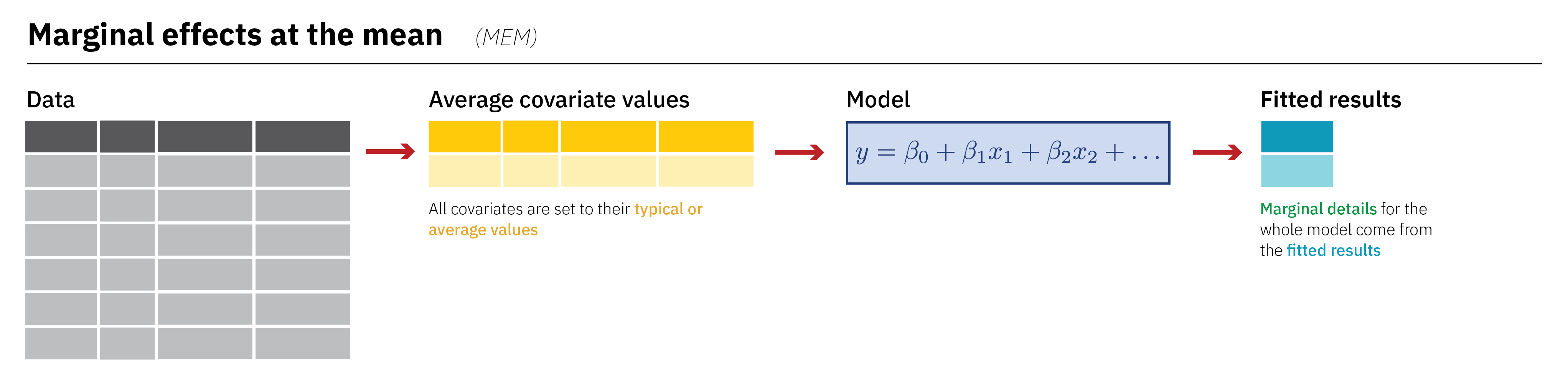
Marginal Effects at the Mean (MEM)
Term Contrast Estimate Std. Error z Pr(>|z|) S
bill_length_mm dY/dX 72.69 10.64 6.8312 <0.001 36.8
flipper_length_mm dY/dX 27.26 3.17 8.5877 <0.001 56.6
species Chinstrap - Adelie -656.05 94.90 -6.9128 <0.001 37.6
species Gentoo - Adelie 3.65 95.21 0.0383 0.969 0.0
2.5 % 97.5 %
51.8 93.5
21.0 33.5
-842.1 -470.0
-183.0 190.3
Columns: rowid, term, contrast, estimate, std.error, statistic, p.value, s.value, conf.low, conf.high, predicted_lo, predicted_hi, predicted, bill_length_mm, species, flipper_length_mm, body_mass_g
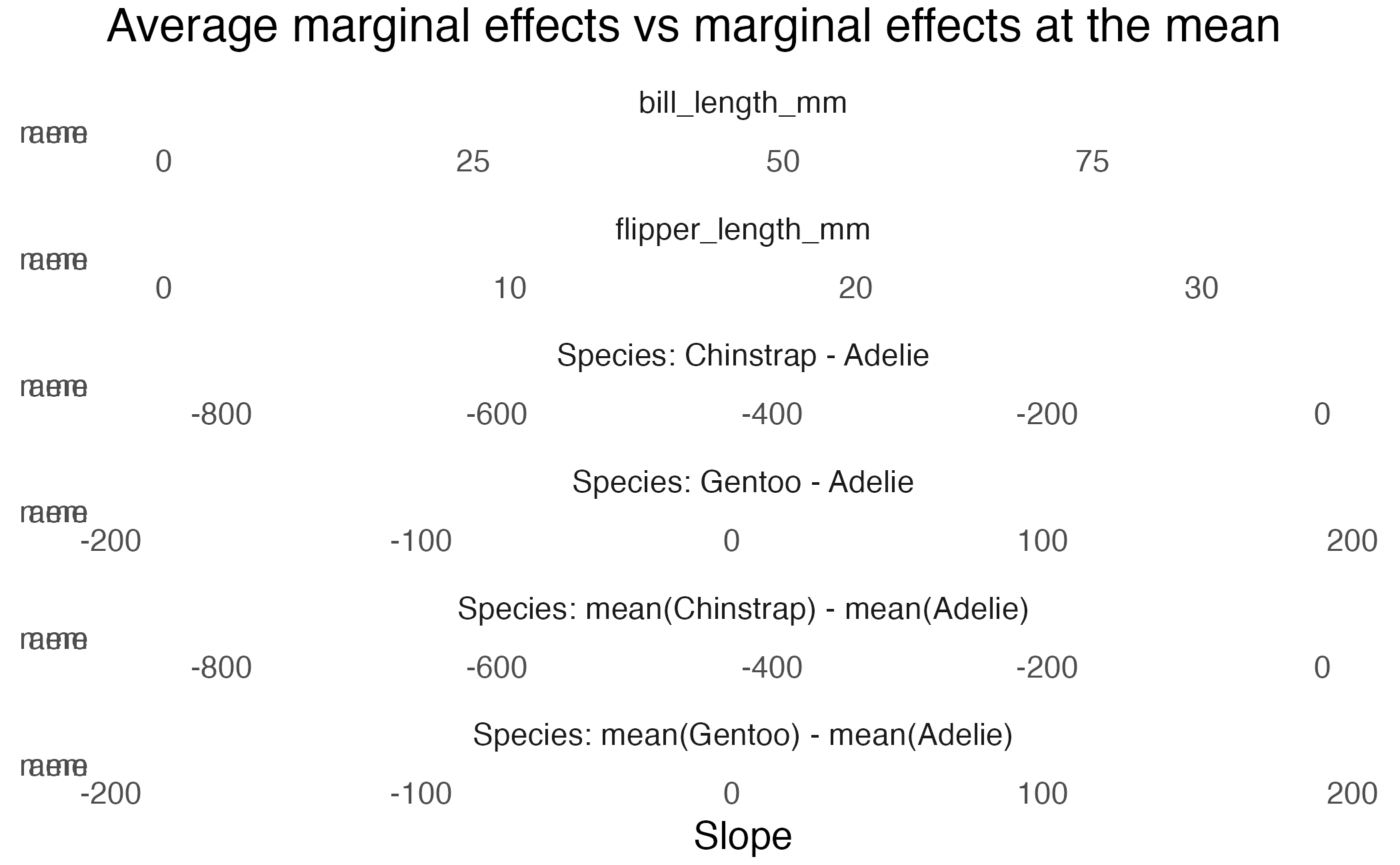
Type: response AME vs MEM
Application exercise
ae-19
- Go to the course GitHub org and find your
ae-19(repo name will be suffixed with your GitHub name). - Clone the repo in RStudio Workbench, open the Quarto document in the repo, and follow along and complete the exercises.
Wrap-up
Wrap-up
- Interpreting and explainin machine learning models is critical for obtaining buy-in from stakeholders.
- White-box models naturally lend themselves to interpretation and explanation.
- Marginal effects can be used to understand the impact of a predictor on the outcome variable.
- Marginal effects are conditional on the underlying data and can be aggregated in various ways.
Acknowledgements and additional resources
- Slides draw on material from The Marginal Effects Zoo and licensed under a Creative Commons Attribution 4.0 International License.
- Additional guide to marginal effects by Andrew Heiss