Optimizing color spaces
Lecture 16
Dr. Benjamin Soltoff
Cornell University
INFO 3312/5312 - Spring 2026
March 20, 2026
Announcements
Announcements
- Homework 05
- Project 02
Uses of color in data visualization
|

|
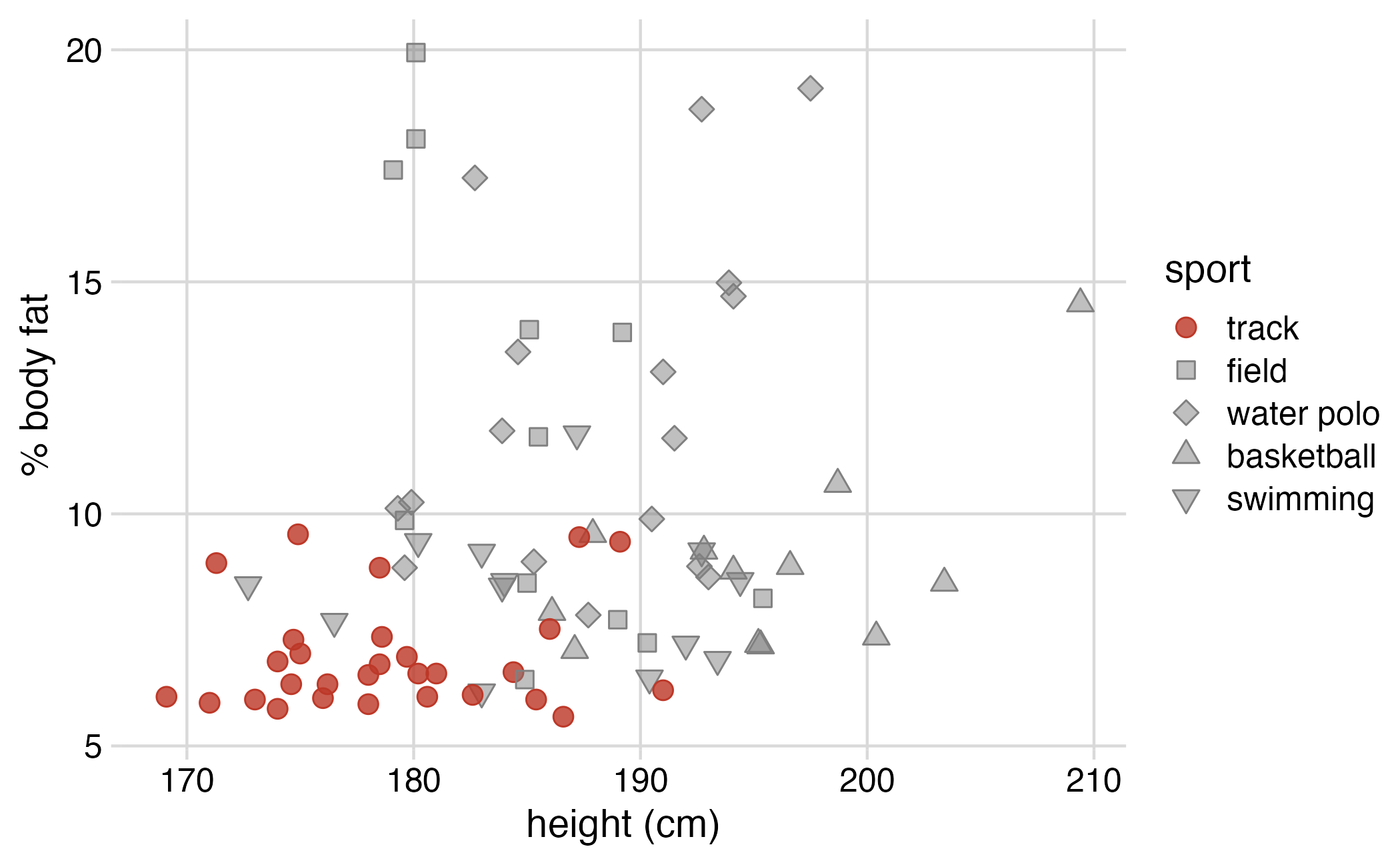
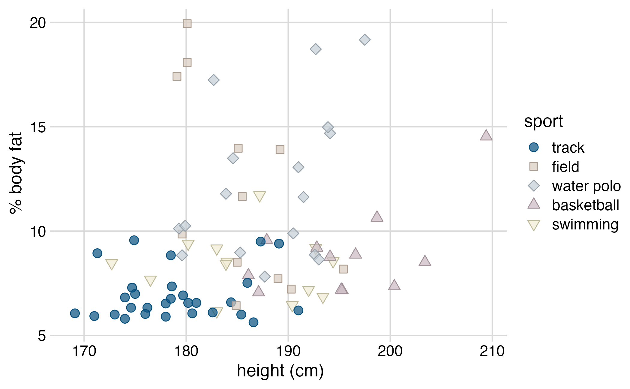
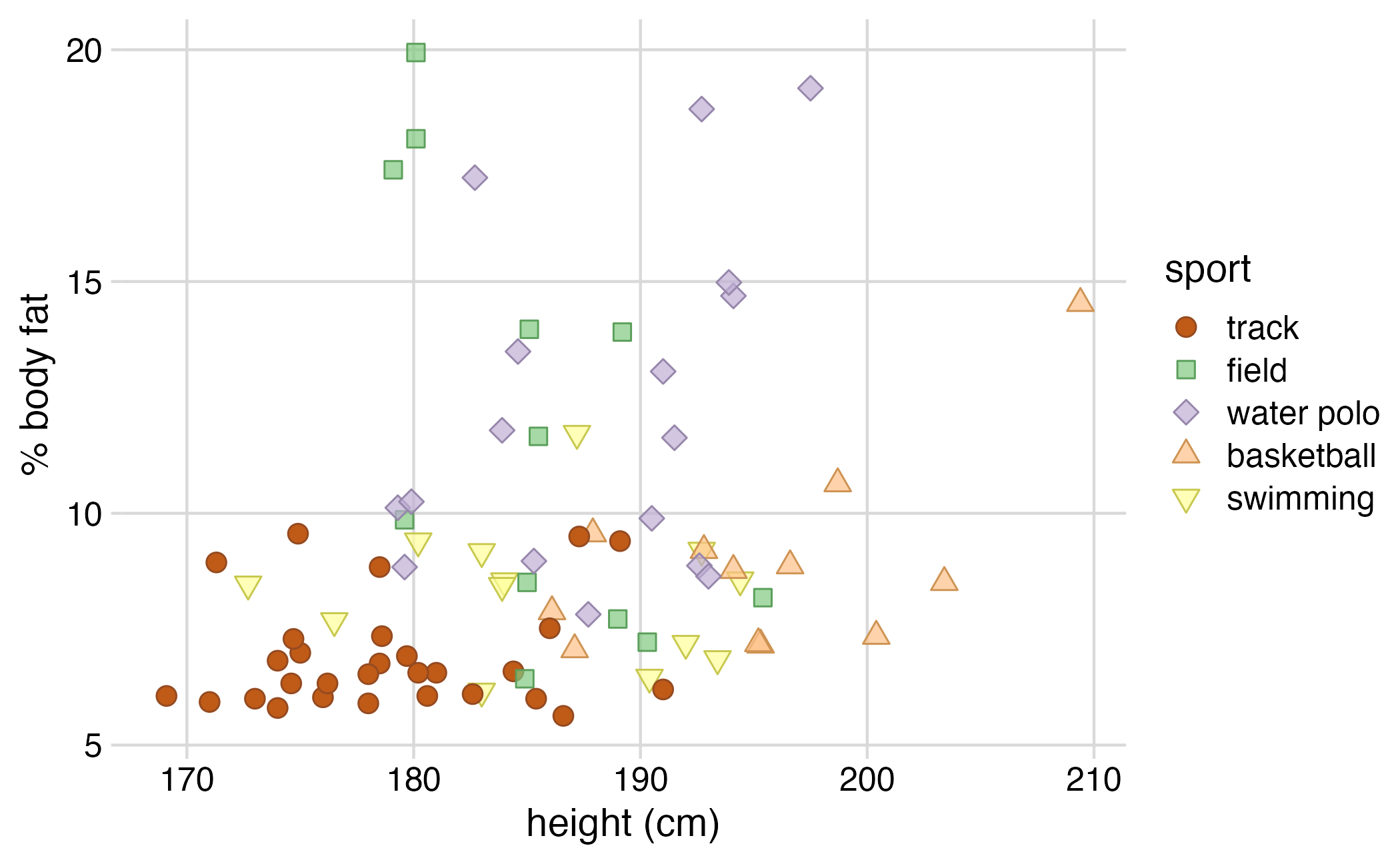
Qualitative scale example
Figure redrawn from Claus O. Wilke. Fundamentals of Data Visualization. O’Reilly, 2019.
Uses of color in data visualization
|

|
|

|
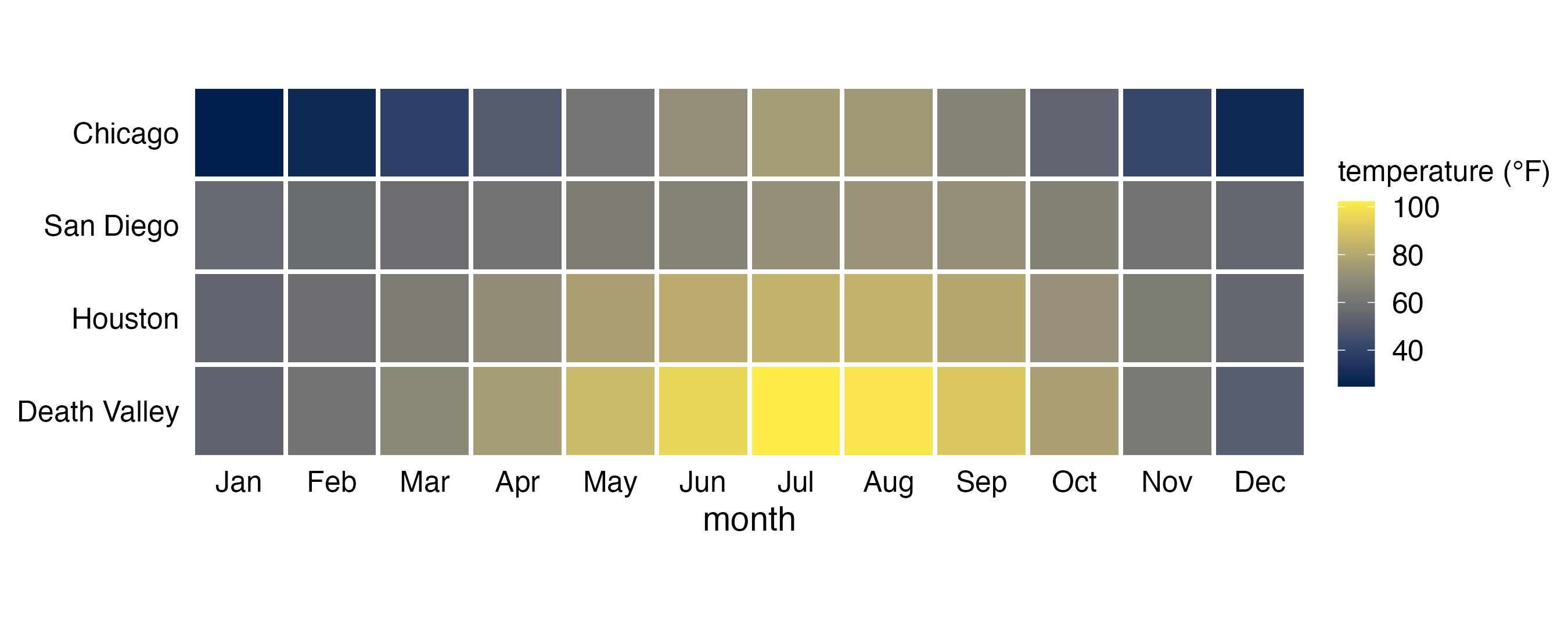
Sequential scale example
Figure redrawn from Claus O. Wilke. Fundamentals of Data Visualization. O’Reilly, 2019.
Uses of color in data visualization
|

|
|

|
|

|
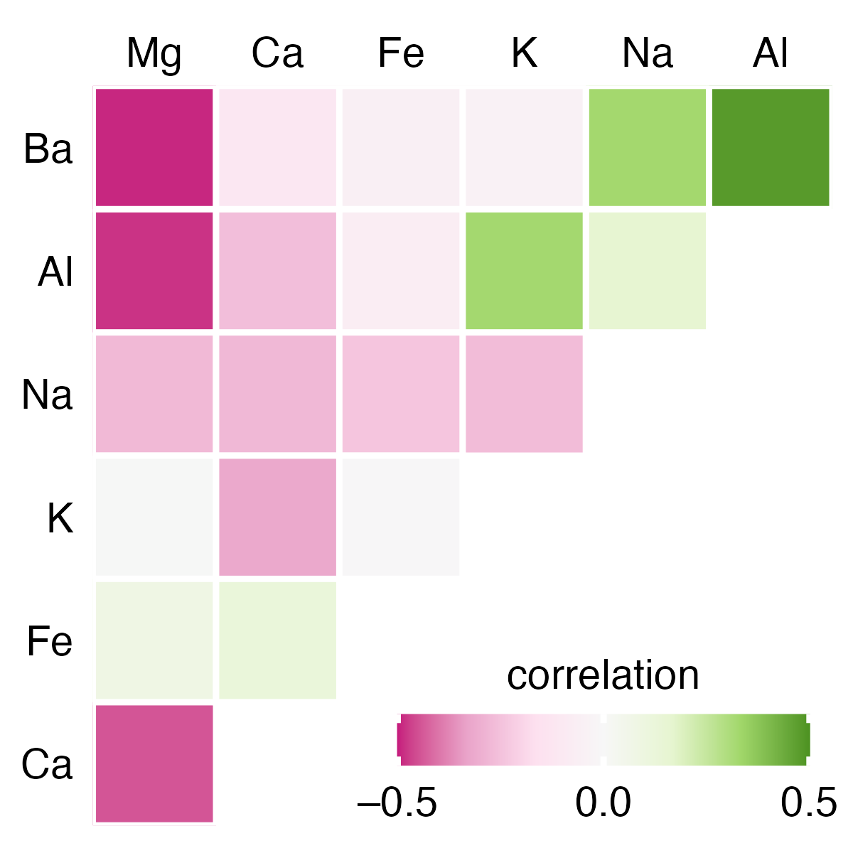
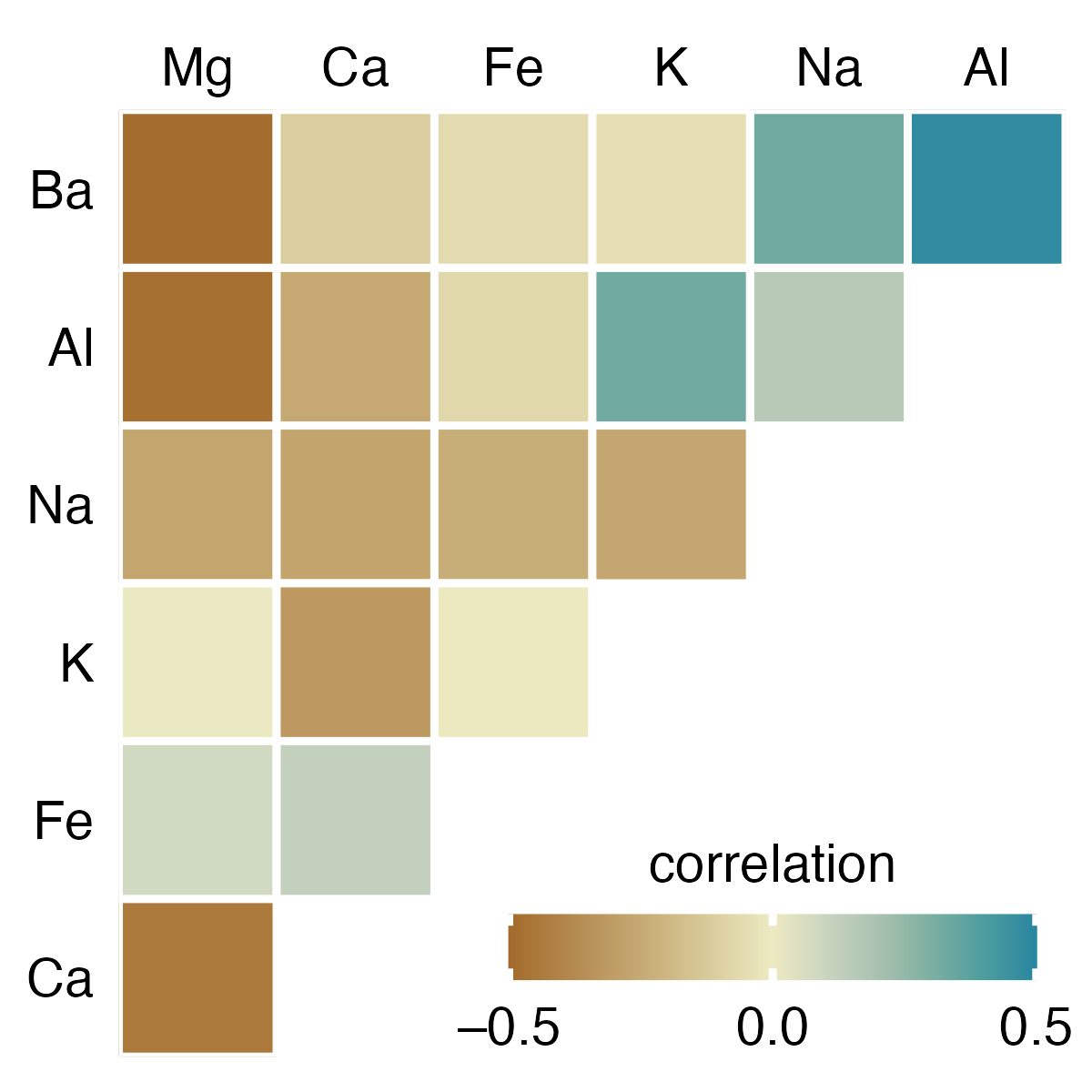
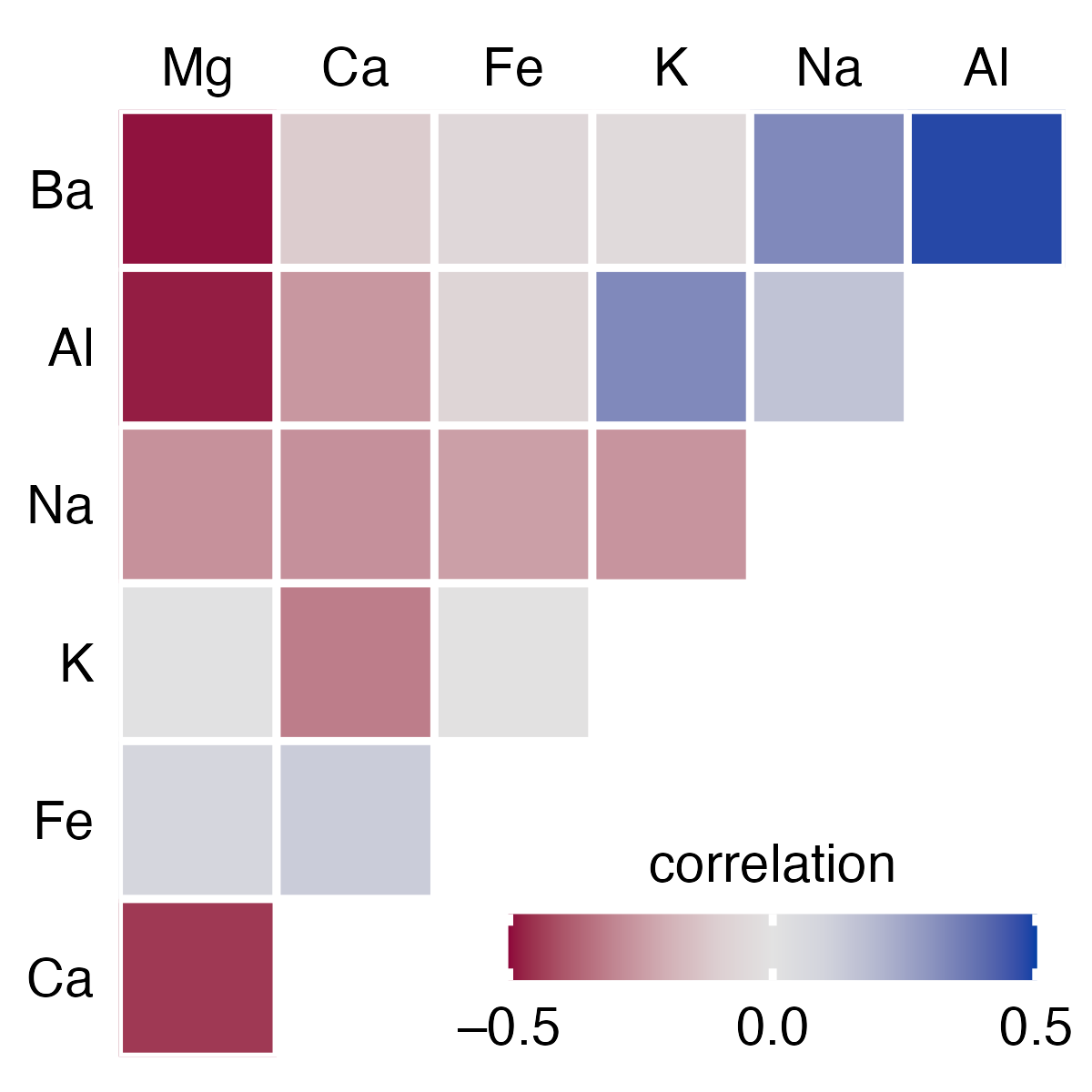
Diverging scale example
Figure redrawn from Claus O. Wilke. Fundamentals of Data Visualization. O’Reilly, 2019.
Uses of color in data visualization
|

|
|

|
|

|
|

|
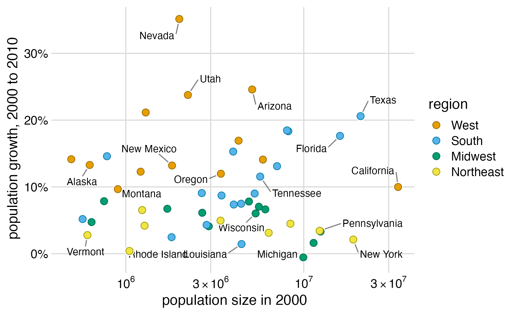
Highlight example
Figure redrawn from Claus O. Wilke. Fundamentals of Data Visualization. O’Reilly, 2019.
Uses of color in data visualization
|

|
|

|
|

|
|

|
Choosing a color scale
Choosing a color scale
- Emphasis on interpretability and accessibility
- Default palettes are less than desirable
- Variables may require transformations
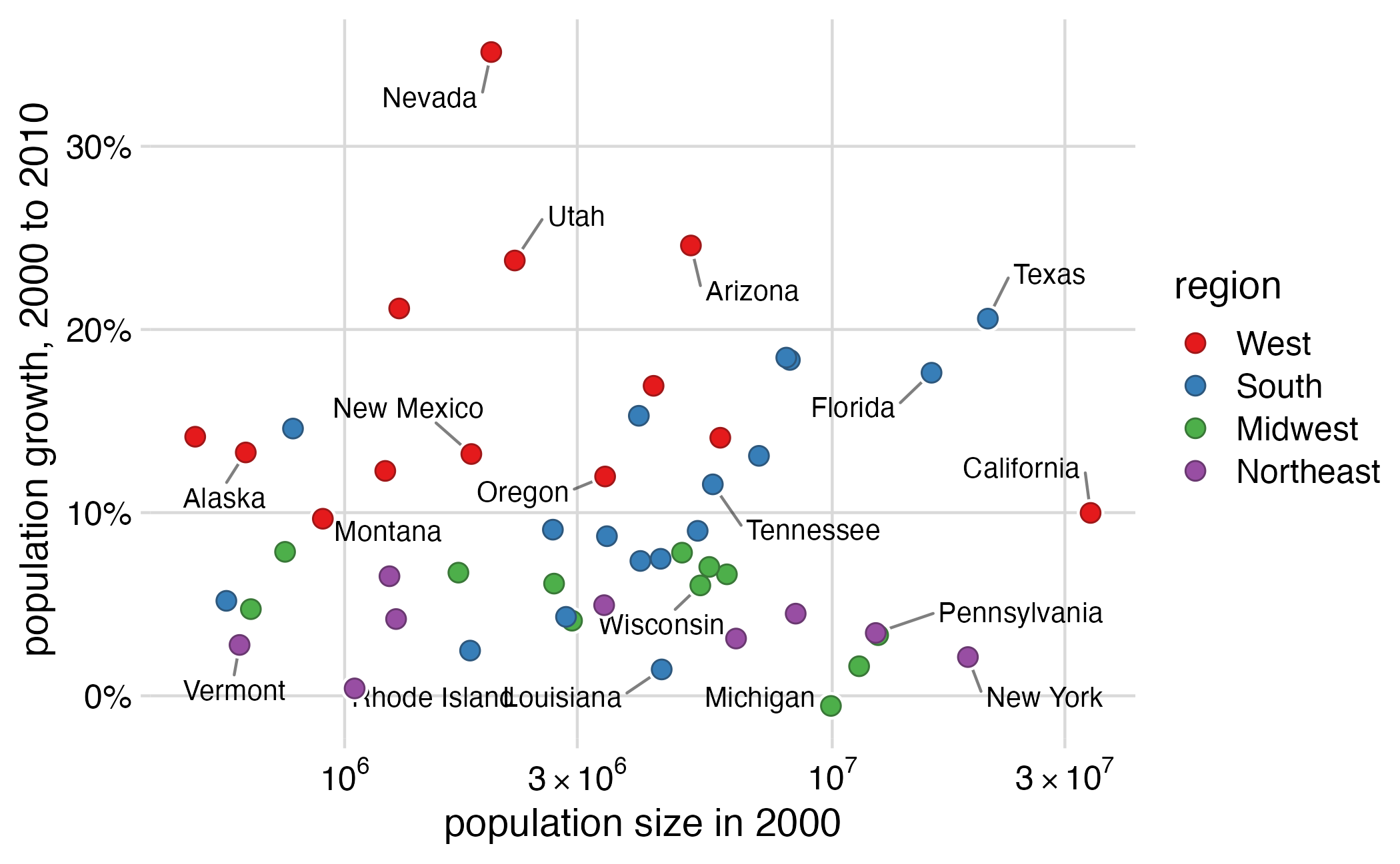
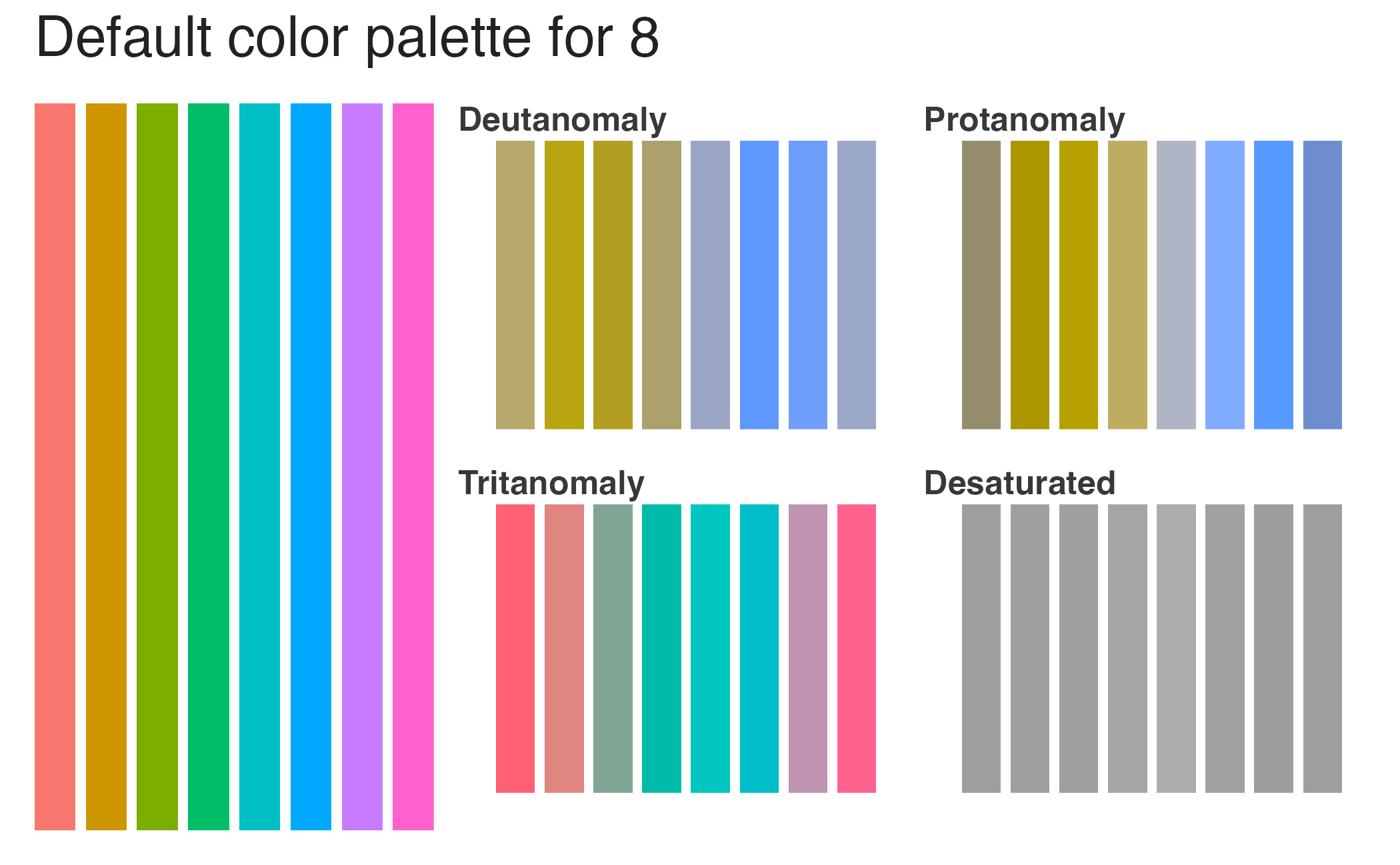
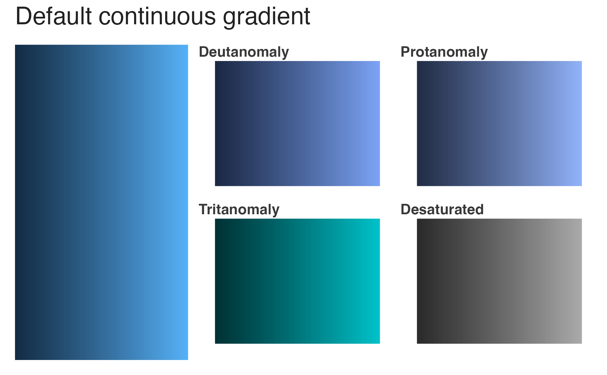
Default palette in {ggplot2}
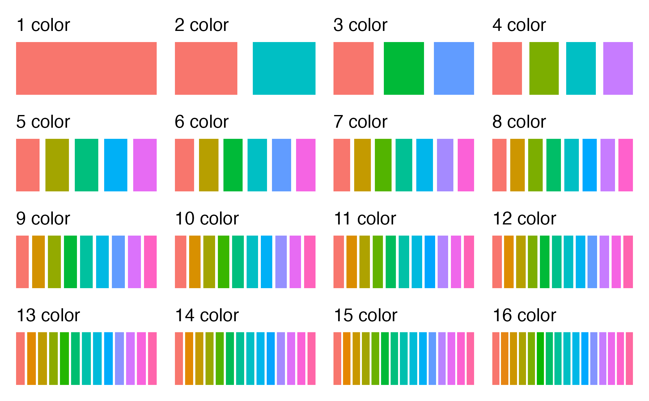
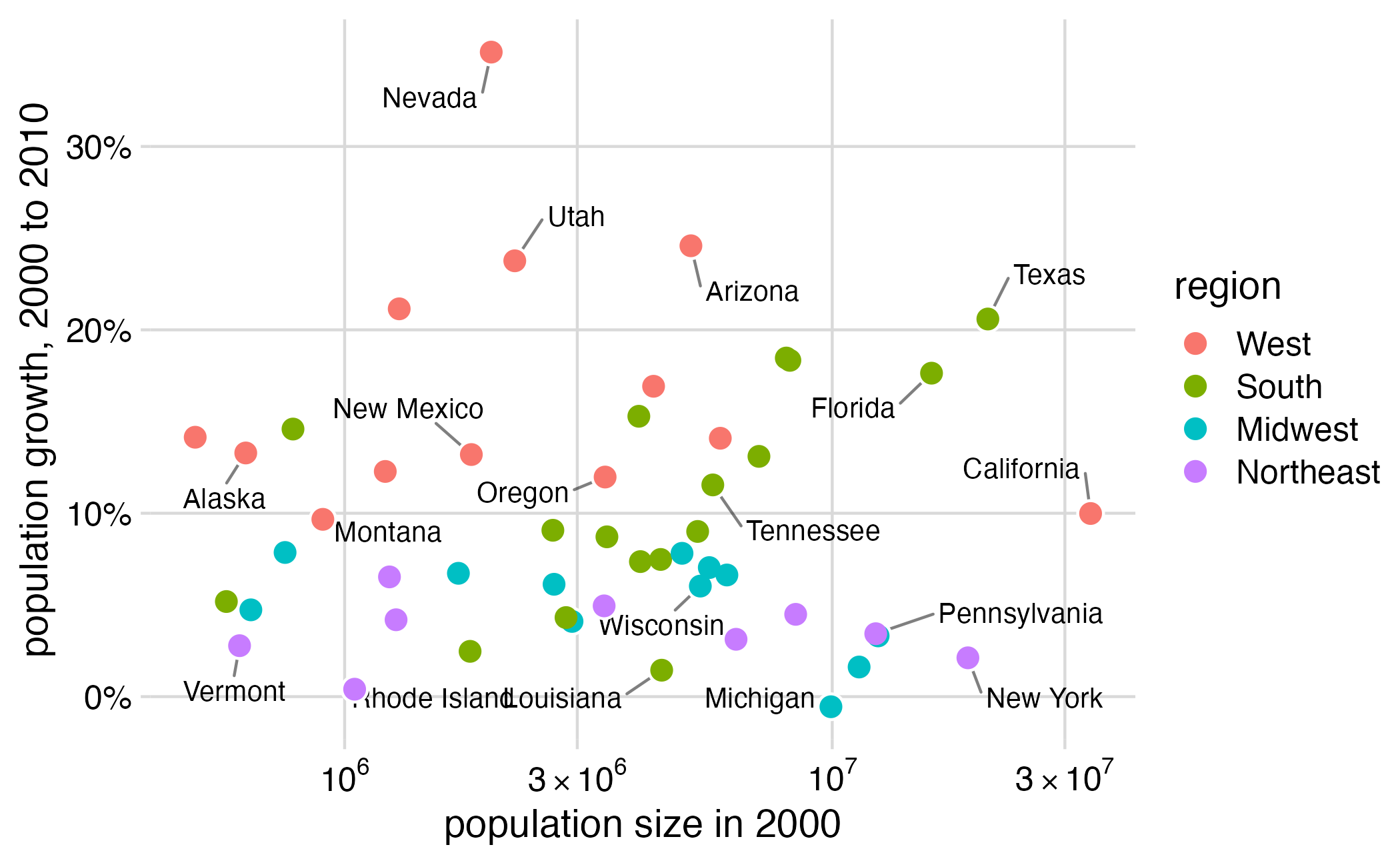
Suboptimal default choices
Common forms of color vision deficiency
Red-green
- Deuteranomaly
- Protanomaly
- Protanopia and deuteranopia
Blue-yellow
- Tritanomaly
- Tritanopia
Complete color vision deficiency
- Monochromacy
Inspecting for color vision deficiency
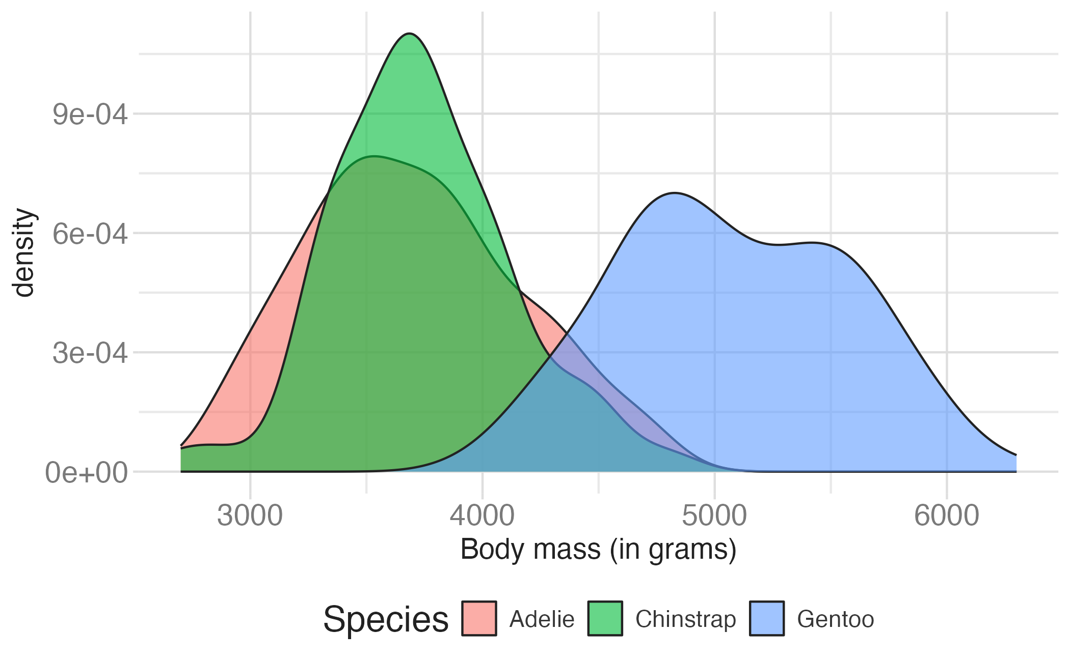
Inspecting for color vision deficiency
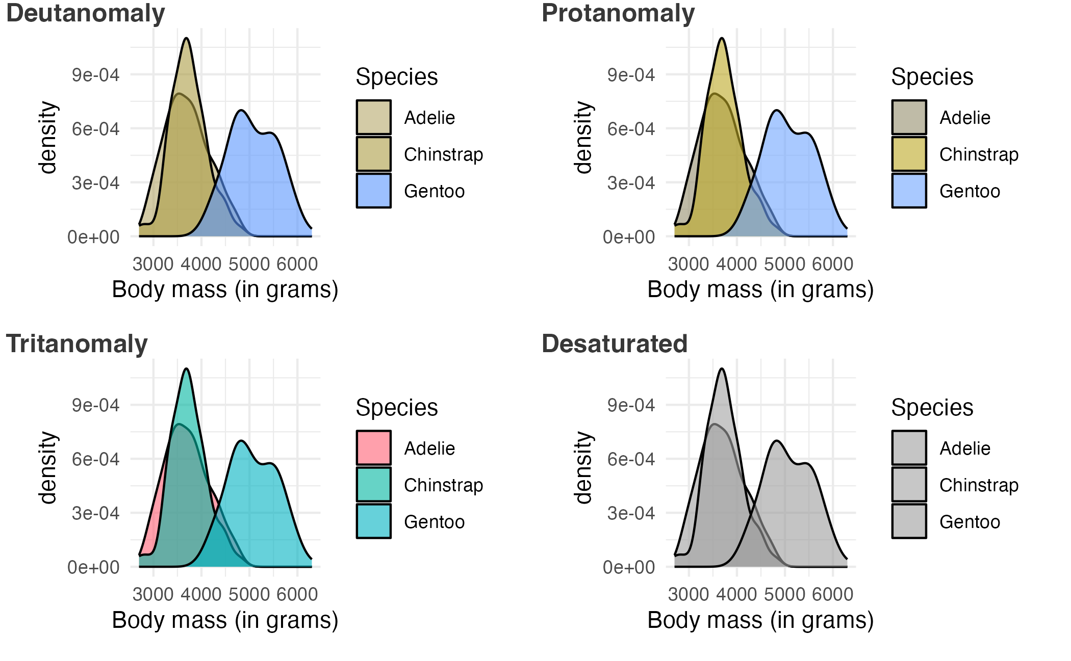
Inspecting for color deficiency
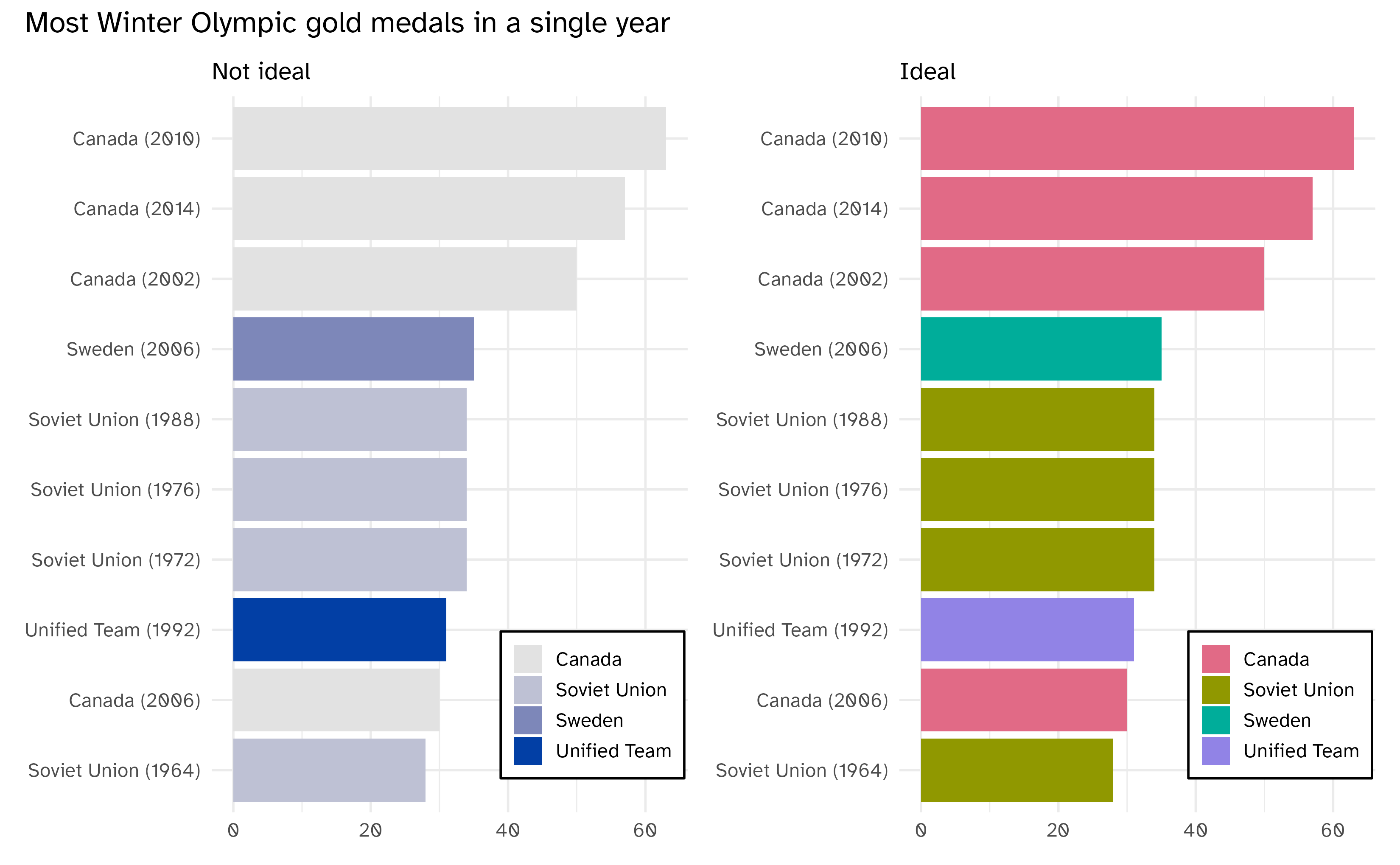
Inspecting for color deficiency
When to use quantitative or qualitative color scales?
Quantitative vs. qualitative palettes
- Quantitative \(\equiv\) numerical
- Qualitative \(\equiv\) categorical

Source: Lisa Charlotte Muth
Use qualitative for nominal variables
Use quantitative for ordinal variables
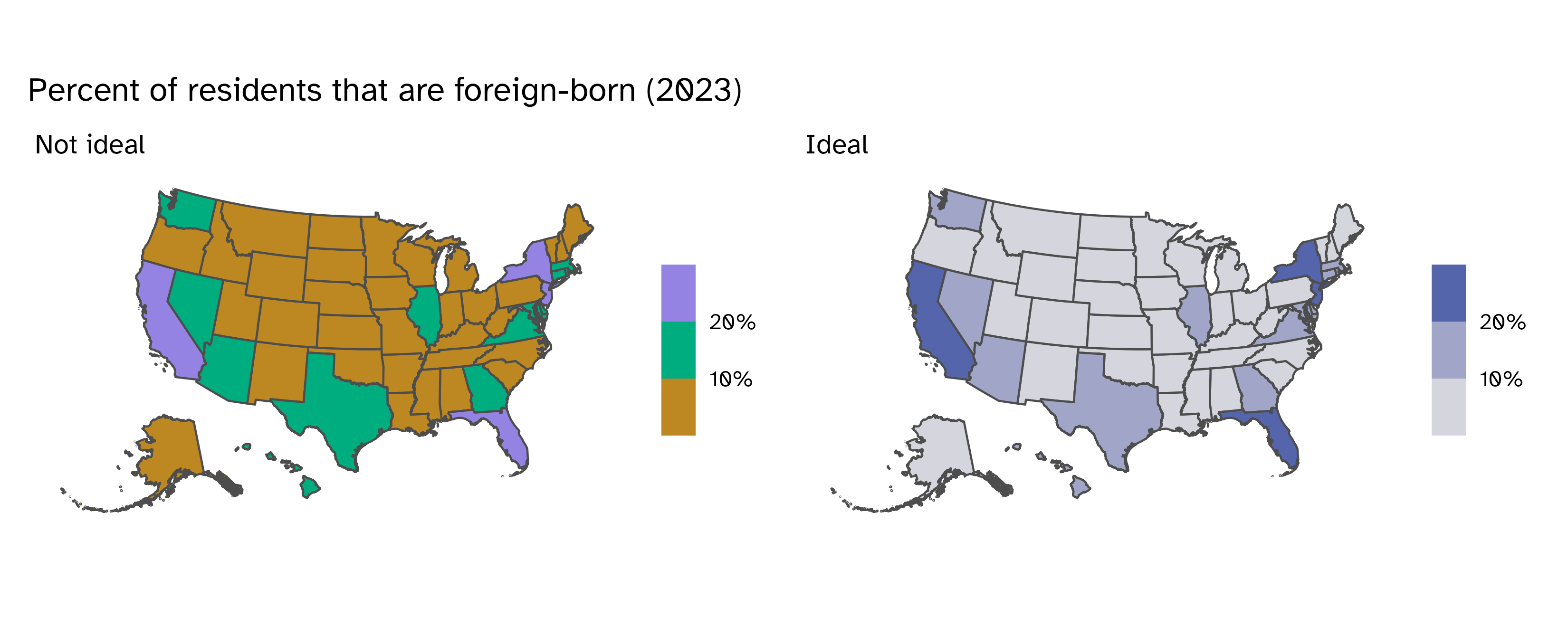
Consider binning continuous variables
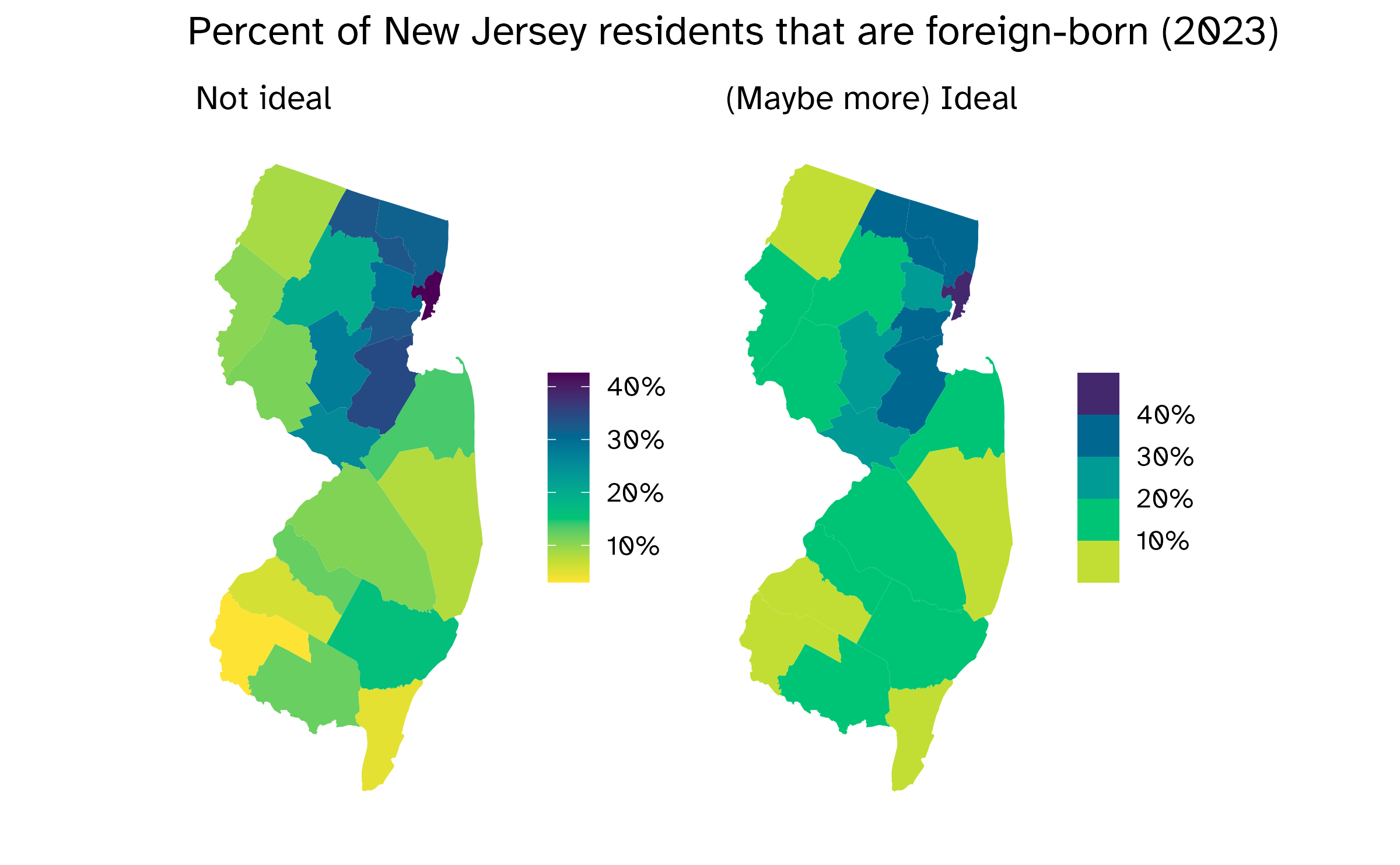
Quantitative \(\neq\) continuous
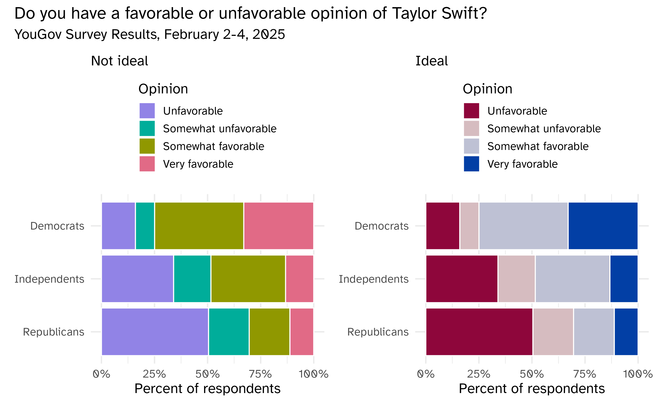
Shades to emphasize order
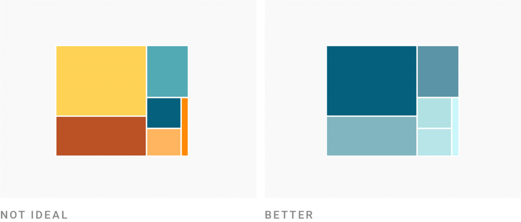
Source: Lisa Charlotte Muth
Shades to distinguish subcategories
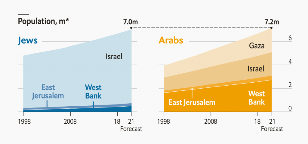
Source: Lisa Charlotte Muth
Implementing optimal color palettes in R
{ggplot2} color scale functions
| Scale function | Aesthetic | Data type | Palette type |
|---|---|---|---|
scale_color_hue() |
color |
discrete | qualitative |
{ggplot2} color scale functions are a bit of a mess
| Scale function | Aesthetic | Data type | Palette type |
|---|---|---|---|
scale_color_hue() |
color |
discrete | qualitative |
scale_fill_hue() |
fill |
discrete | qualitative |
{ggplot2} color scale functions are a bit of a mess
| Scale function | Aesthetic | Data type | Palette type |
|---|---|---|---|
scale_color_hue() |
color |
discrete | qualitative |
scale_fill_hue() |
fill |
discrete | qualitative |
scale_color_gradient() |
color |
continuous | sequential |
{ggplot2} color scale functions are a bit of a mess
| Scale function | Aesthetic | Data type | Palette type |
|---|---|---|---|
scale_color_hue() |
color |
discrete | qualitative |
scale_fill_hue() |
fill |
discrete | qualitative |
scale_color_gradient() |
color |
continuous | sequential |
scale_color_gradient2() |
color |
continuous | diverging |
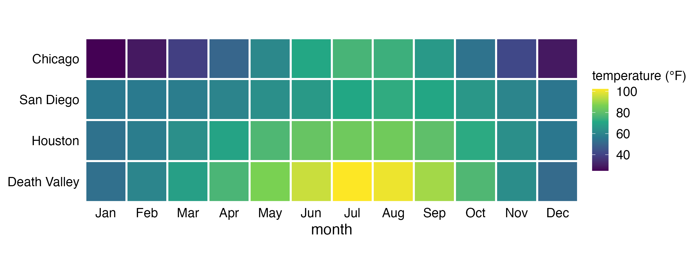
scale_fill_viridis_c() |
color |
continuous | sequential |
scale_fill_viridis_d() |
fill |
discrete | sequential |
scale_color_brewer() |
color |
discrete | qualitative, diverging, sequential |
scale_fill_brewer() |
fill |
discrete | qualitative, diverging, sequential |
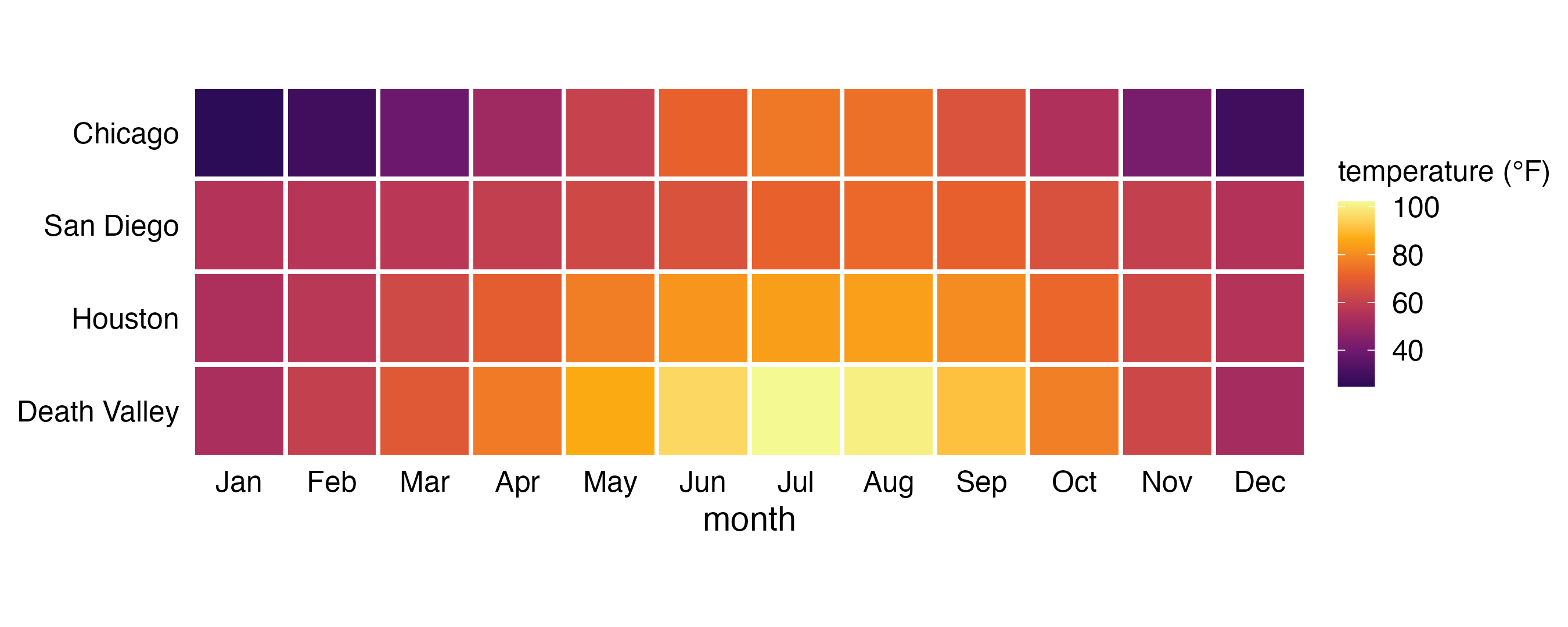
scale_color_distiller() |
color |
continuous | qualitative, diverging, sequential |
… and there are many many more
Examples

Examples

Examples

Examples

Examples

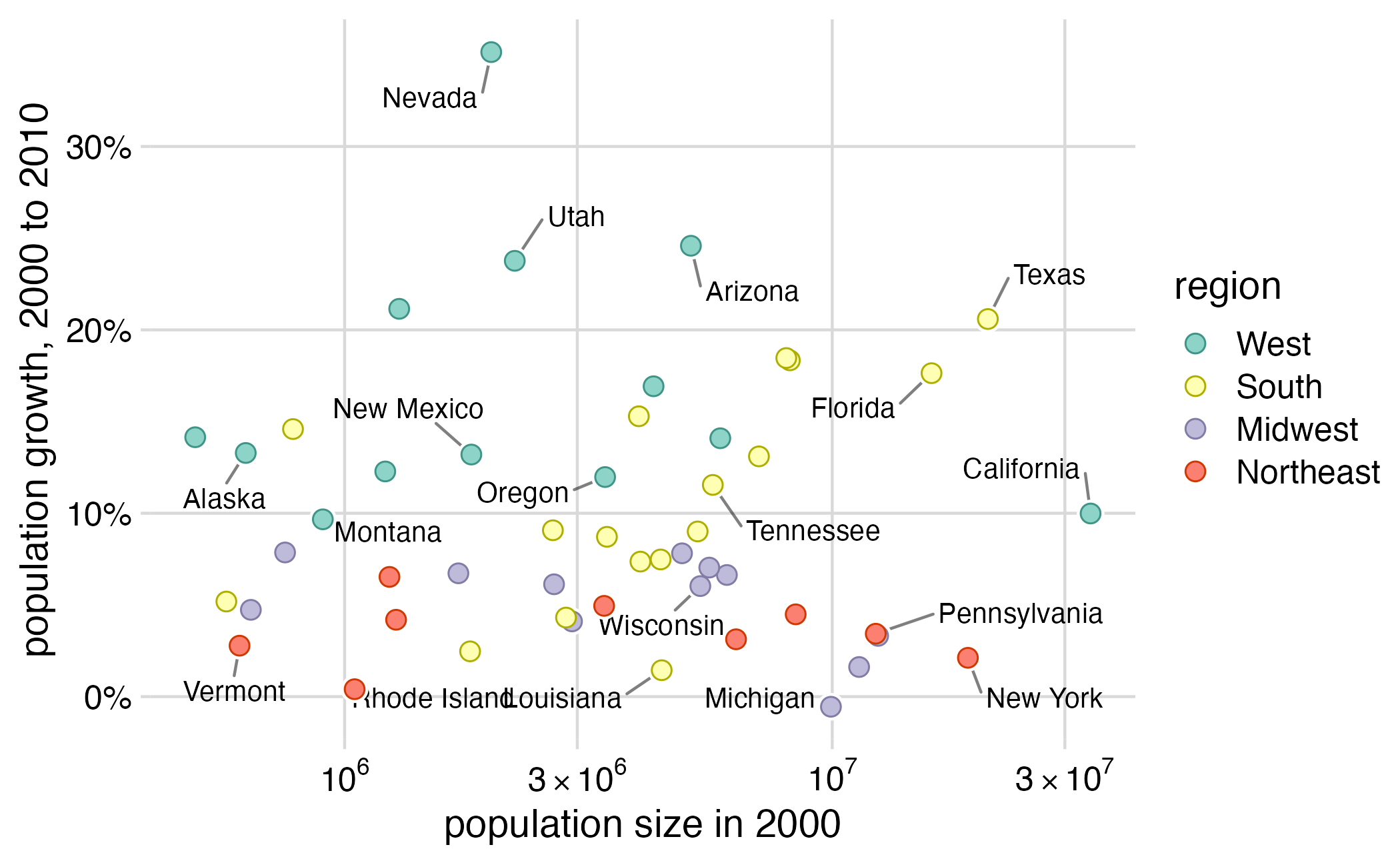
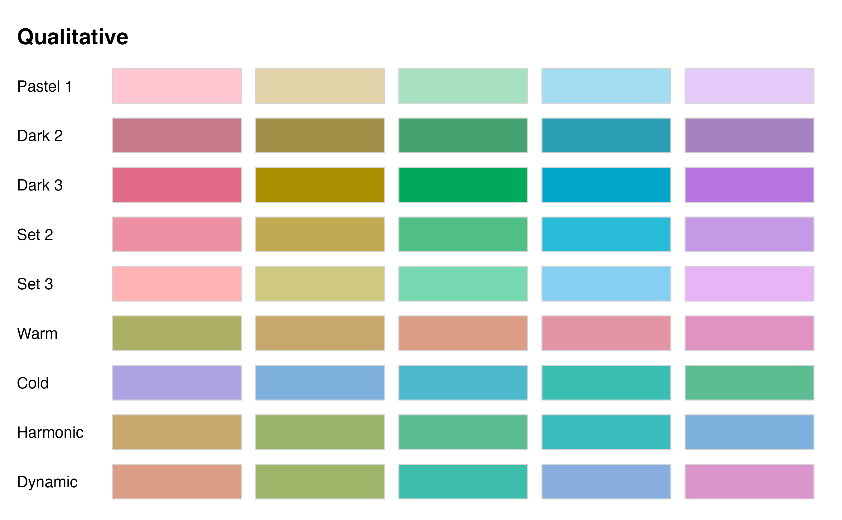
The {colorspace} package creates some order
Scale name: scale_<aesthetic>_<datatype>_<colorscale>()
<aesthetic>: name of the aesthetic (fill,color)<datatype>: type of variable plotted (discrete,continuous,binned)<colorscale>: type of the color scale (qualitative,sequential,diverging,divergingx)
| Scale function | Aesthetic | Data type | Palette type |
|---|---|---|---|
scale_color_discrete_qualitative() |
color |
discrete | qualitative |
scale_fill_continuous_sequential() |
fill |
continuous | sequential |
scale_colour_continuous_divergingx() |
colour |
continuous | diverging |
Examples

Examples

Examples

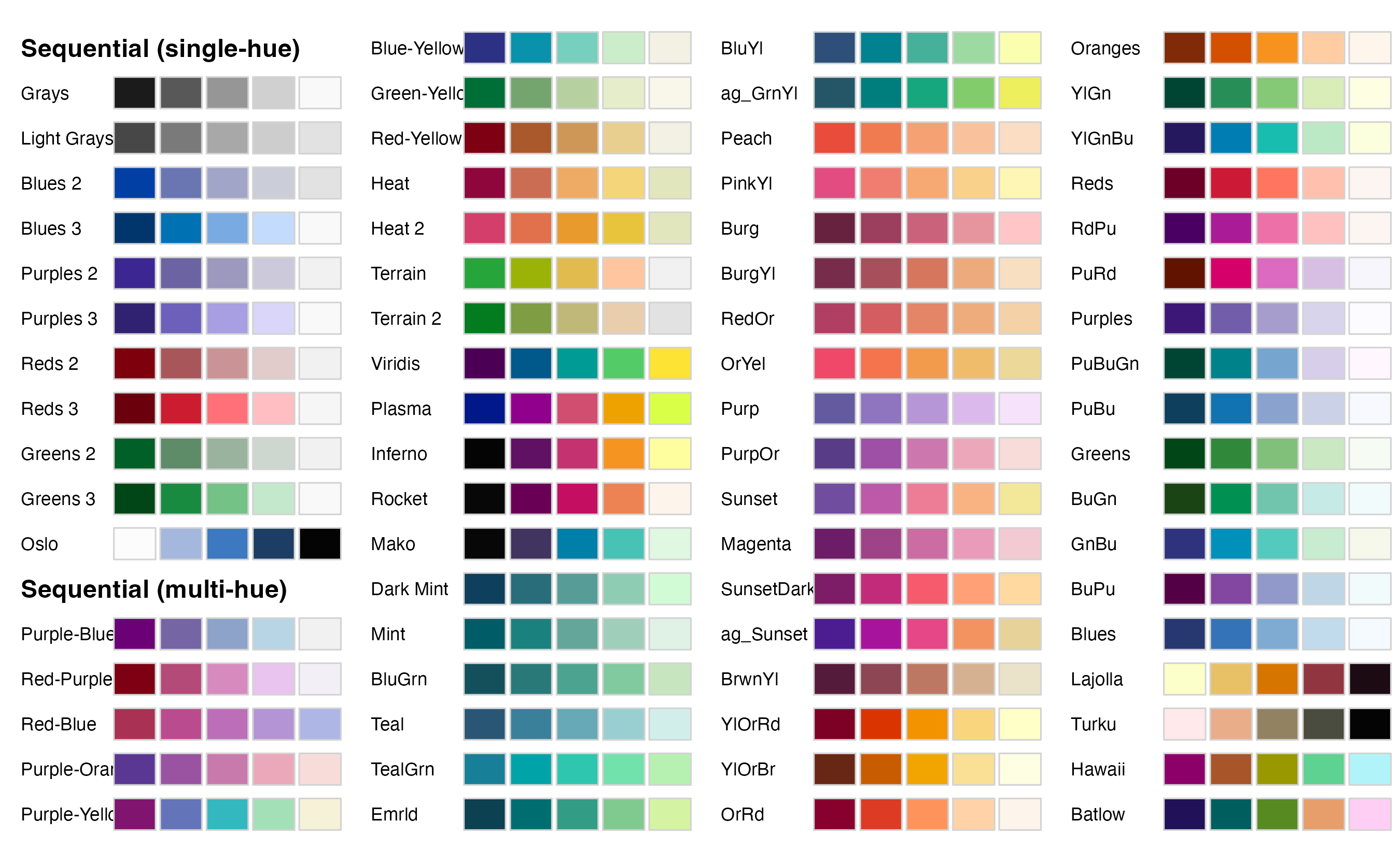
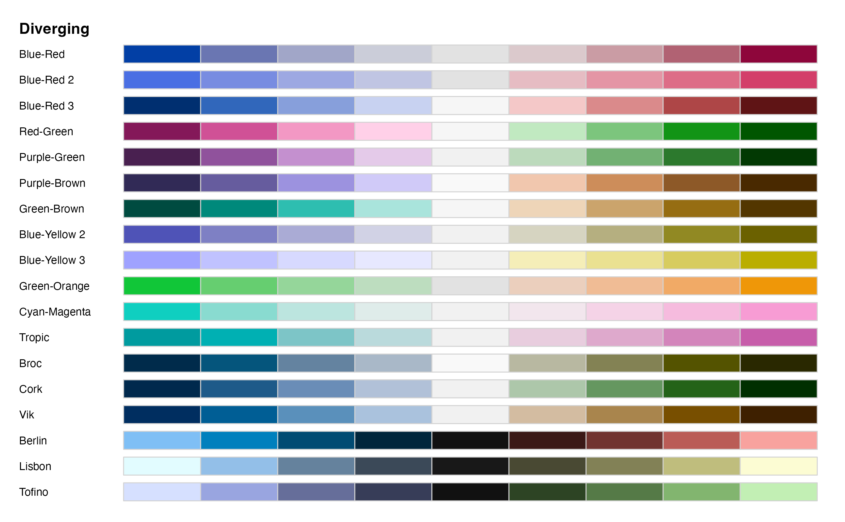
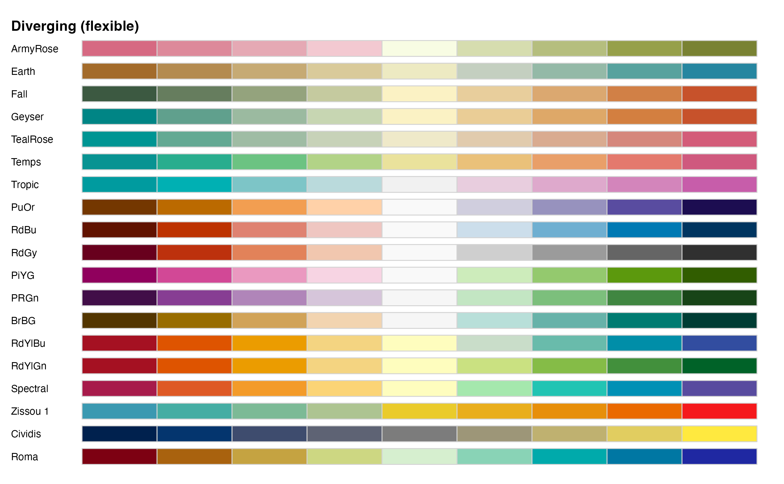
Setting colors for discrete, qualitative scales
Examples

Examples
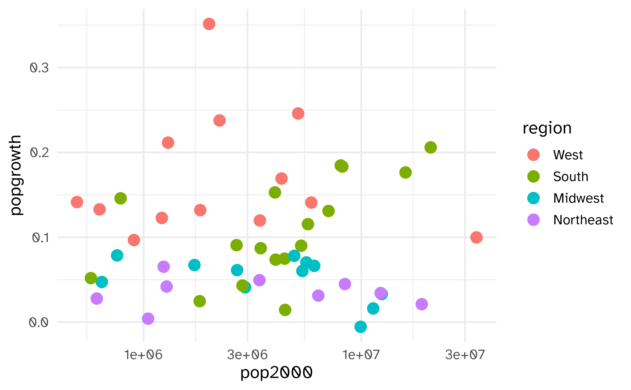
Examples
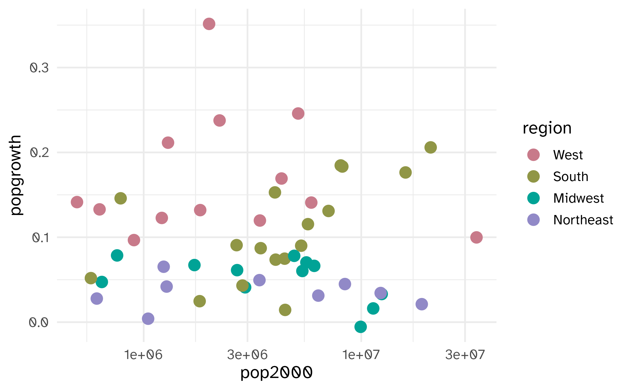
Examples
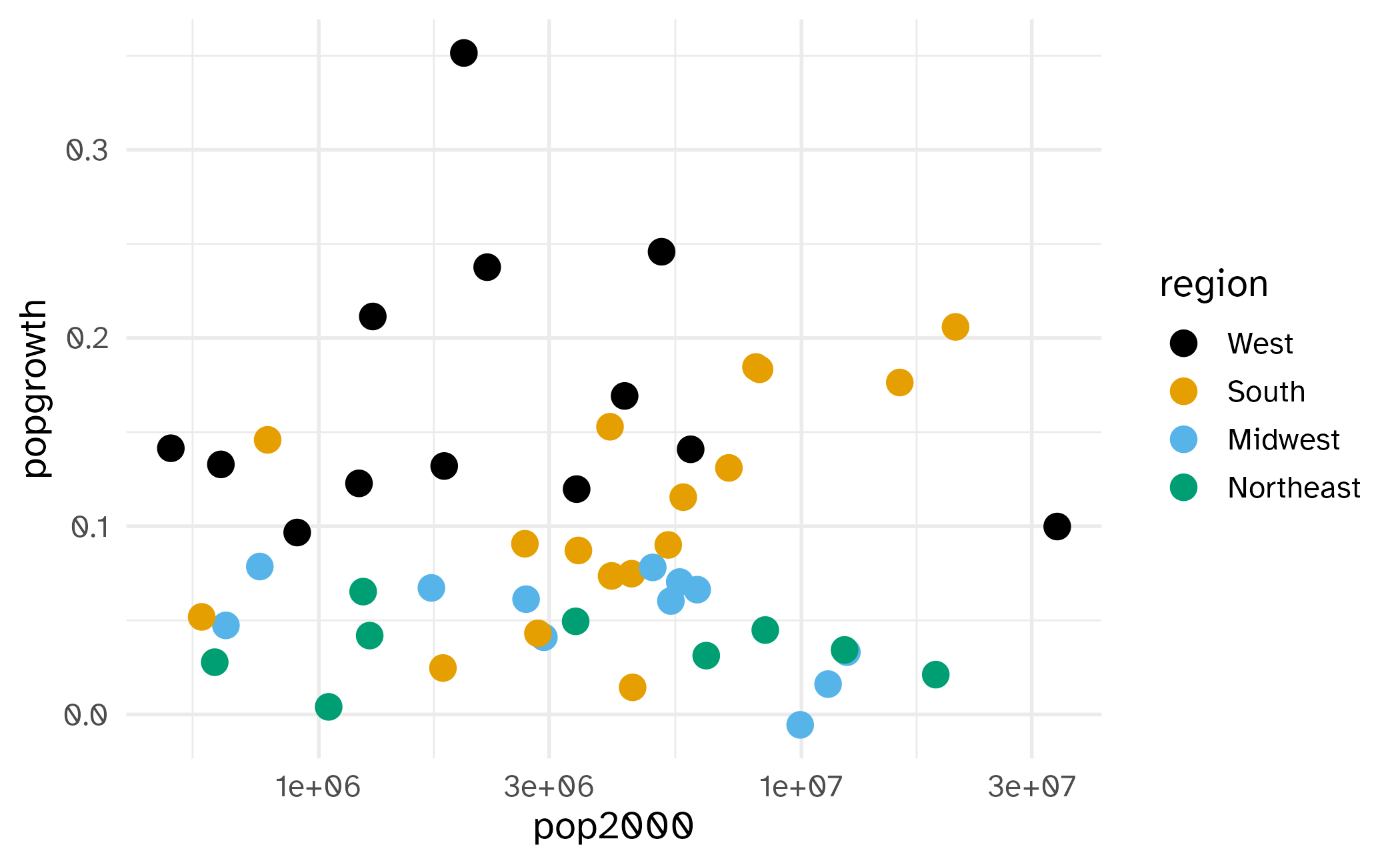
Examples
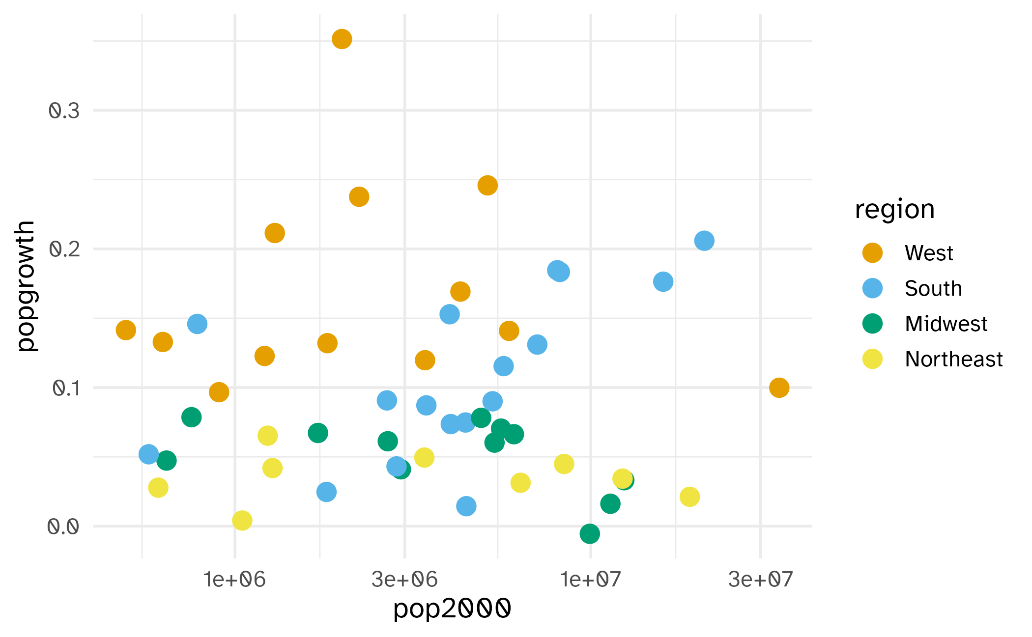
Okabe-Ito RGB codes

| Name | Hex code | R, G, B (0-255) |
|---|---|---|
| orange | #E69F00 | 230, 159, 0 |
| sky blue | #56B4E9 | 86, 180, 233 |
| bluish green | #009E73 | 0, 158, 115 |
| yellow | #F0E442 | 240, 228, 66 |
| blue | #0072B2 | 0, 114, 178 |
| vermilion | #D55E00 | 213, 94, 0 |
| reddish purple | #CC79A7 | 204, 121, 167 |
| black | #000000 | 0, 0, 0 |
Application exercise
ae-15
Instructions
- Go to the course GitHub org and find your
ae-15(repo name will be suffixed with your GitHub name). - Clone the repo in Positron, run
renv::restore()to install the required packages, open the Quarto document in the repo, and follow along and complete the exercises. - Render, commit, and push your edits by the AE deadline – end of the day
Wrap up
Recap
- Color is a powerful tool in data visualization
- Use color to distinguish categories and represent numeric values
- Choose color scales that are interpretable and accessible
- Use qualitative scales for nominal variables
- Use quantitative scales for numeric/ordinal variables
- Consider binning continuous variables
