-- geo_export_6fd95df5-1136-4829-8f2d-9cb5d1cc2222.dbf
-- geo_export_6fd95df5-1136-4829-8f2d-9cb5d1cc2222.prj
-- geo_export_6fd95df5-1136-4829-8f2d-9cb5d1cc2222.shp
-- geo_export_6fd95df5-1136-4829-8f2d-9cb5d1cc2222.shxVisualizing spatial data II
Lecture 14
March 14, 2024
Spring is just around the corner – or is it already here?
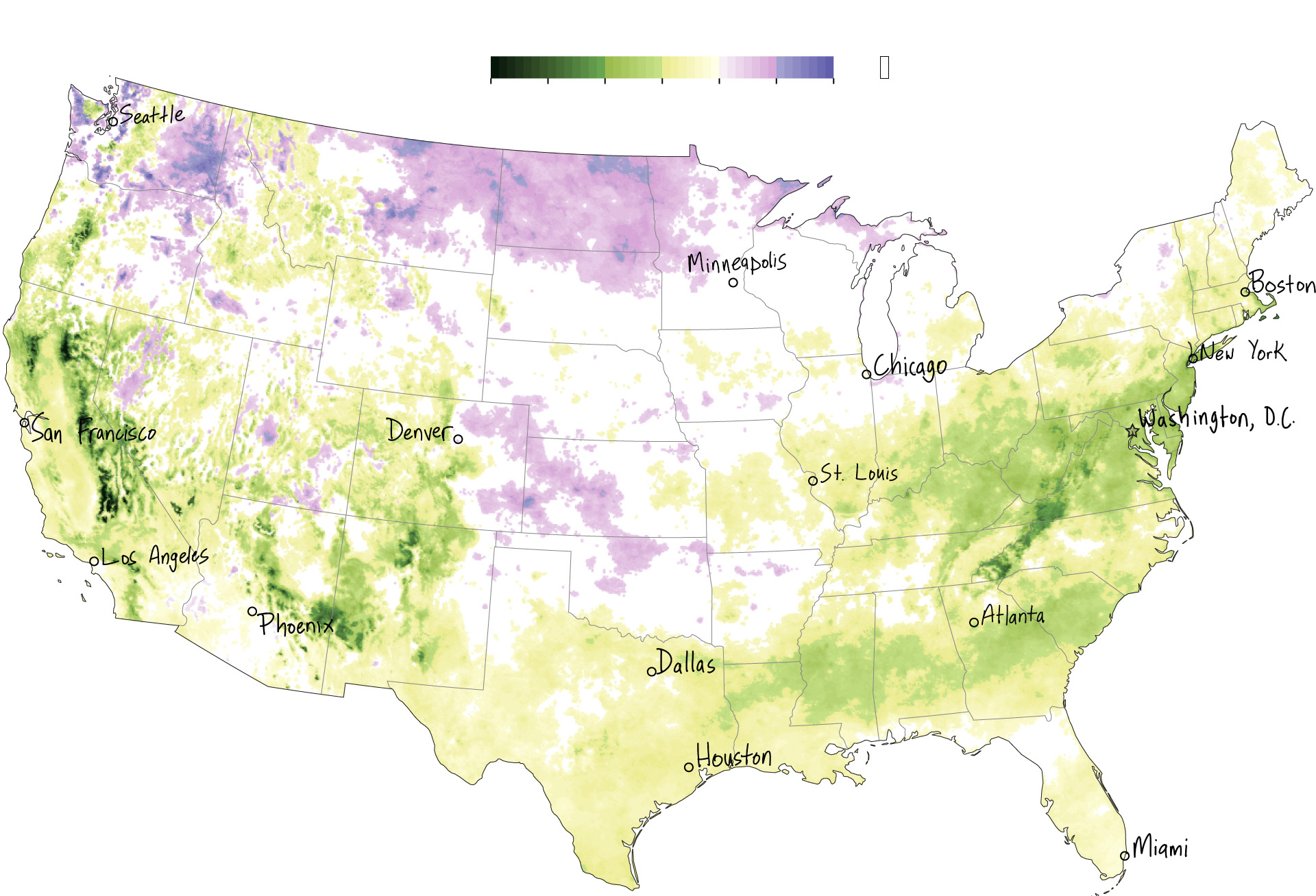
- What is the story?
- How do the aesthetic design choices support the story?
Simple Features for R
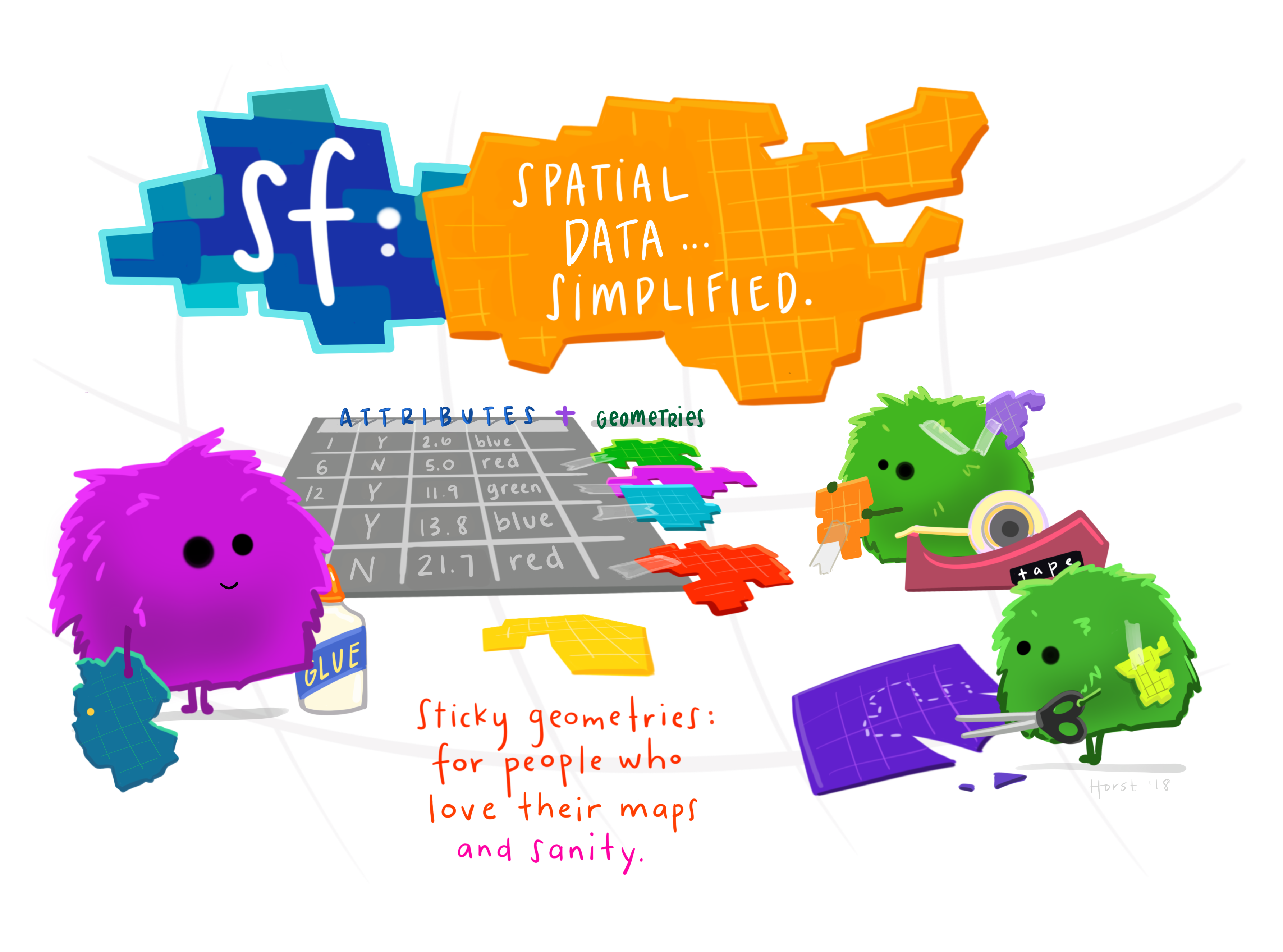
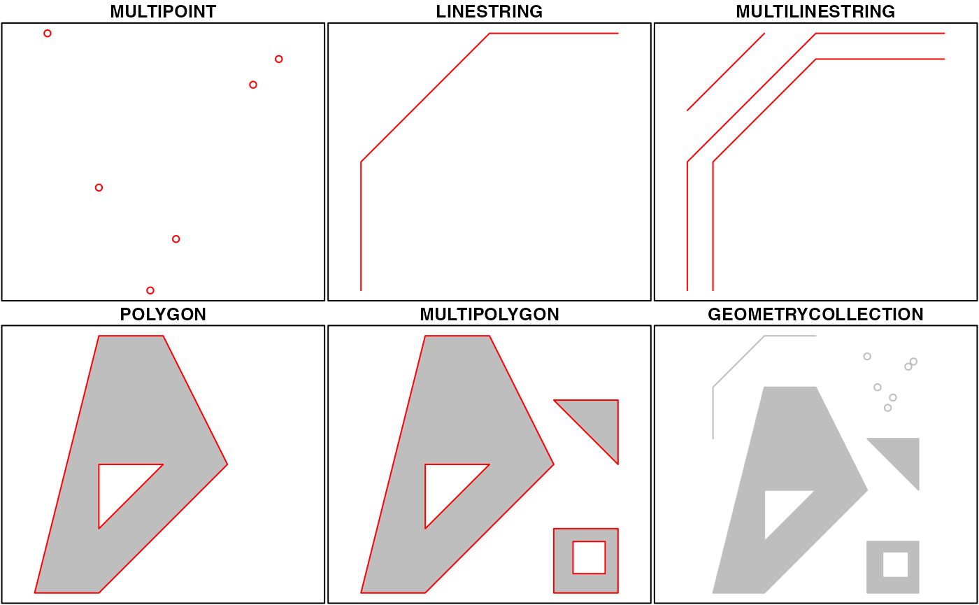
Simple features
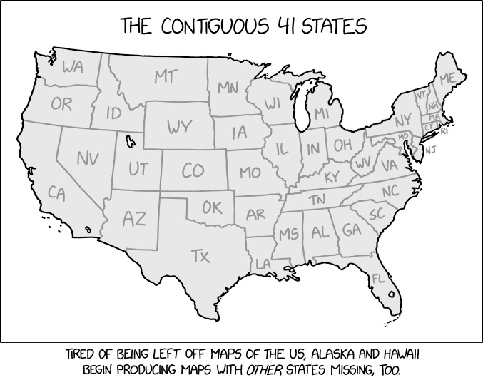
USA boundaries

Plot a subset of a map

Just another ggplot()

urbnmapr

Points

Points

Plotting with two sf data frames

Choropleths

Draw the map

Use better colors

Spatial aggregation

Which is better for comparisons?

cut_interval()

cut_number()

ggplot2::binned_scale()

ggplot2::binned_scale() with quartiles

ggplot2::binned_scale() with quartiles

Map projection
Mercator projection

Projection using standard lines

South on the top

Adjusting color intervals and projections

Wrap-up
- Structure geographic features using vector data and simple features
- Use
geom_sf()to visualize simple features data in ggplot2 - Consider spatially aggregating your observations for more effective communication
- Deliberately select color palettes and projection methods
