Visualizing spatial data I

Lecture 13

Dr. Benjamin Soltoff

Cornell University
INFO 3312/5312 - Spring 2024

March 12, 2024

Announcements

Announcements

• Homework 04
• Project 02

Visualization critique

A review of executions in the United States

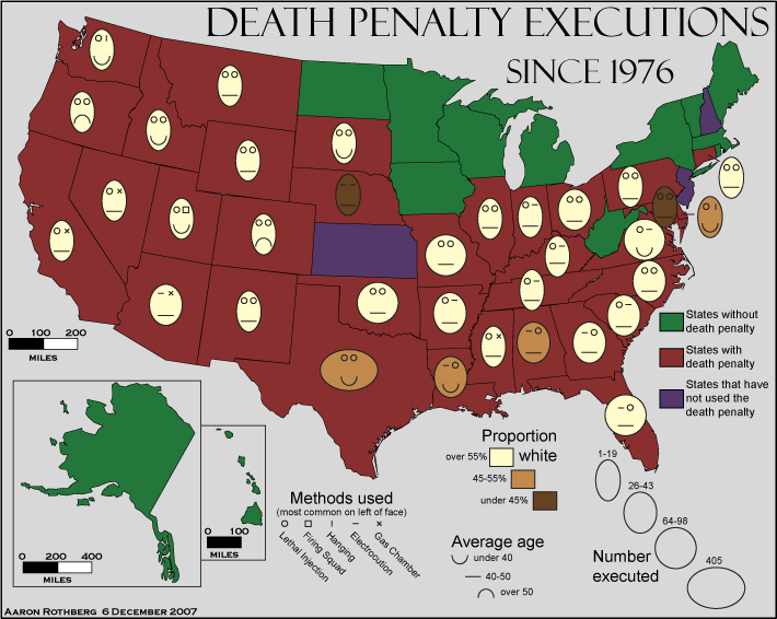
• What is the story?
• What are the design challenges?

Source: Aaron Rothberg

Geospatial visualizations

Geospatial visualizations

• Earliest form of information visualizations
• Geospatial data visualizations
• Google Maps

Not that Jon Snow

Dr. John Snow

Source: Wikipedia

Designing modern maps

• Depict spatial features
• Incorporate additional attributes and information
• Major features
  • Scale
  • Projection
  • Symbols

Scale

• Proportion between distances and sizes on a map and their actual distances and sizes on Earth
• Small-scale map
• Large-scale map

Large-scale map

Small-scale map

Asgard

Midgard

Not flat

Projection

• Process of taking a three-dimensional object and visualizing it on a two-dimensional surface
• No 100% perfect method for this
• Always introduces distortions

Properties of projection methods

1. Shape
2. Area
3. Angles
4. Distance
5. Direction

Symbols

ggmap for raster maps

ggmap

• Package for drawing maps using ggplot2 and raster map tiles
• Static image files generated by mapping services
• Focus on incorporating data into existing maps
• Severely limits ability to change the appearance of the geographic map
• Don’t have to worry about the maps, just the data to go on top

Bounding box

nyc_bb <- c(
  left = -74.263045,
  bottom = 40.487652,
  right = -73.675963,
  top = 40.934743
)

nyc_stamen <- get_stadiamap(
  bbox = nyc_bb,
  zoom = 11
)

ggmap(nyc_stamen)

Level of detail

Identifying bounding box

Use bboxfinder.com to determine the exact longitude/latitude coordinates for the bounding box you wish to obtain.

Types of map tiles

Import crime data

• New York City open data portal
• Crime data from 2022

crimes <- read_csv("data/nyc-crimes.csv")

glimpse(crimes)

Rows: 256,797
Columns: 7
$ cmplnt_num   <chr> "247350382", "243724728", "246348713", "240025455", "2461…
$ boro_nm      <chr> "BROOKLYN", "QUEENS", "QUEENS", "BROOKLYN", "BRONX", "BRO…
$ cmplnt_fr_dt <dttm> 1011-05-18 04:56:02, 1022-04-11 04:56:02, 1022-06-08 04:…
$ law_cat_cd   <chr> "MISDEMEANOR", "MISDEMEANOR", "MISDEMEANOR", "FELONY", "F…
$ ofns_desc    <chr> "CRIMINAL MISCHIEF & RELATED OF", "PETIT LARCENY", "PETIT…
$ latitude     <dbl> 40.66904, 40.77080, 40.68766, 40.65421, 40.83448, 40.6973…
$ longitude    <dbl> -73.90619, -73.81115, -73.83406, -73.95957, -73.85637, -7…

Plot high-level map of crime

nyc <- nyc_stamen
ggmap(nyc)

Using geom_point()

ggmap(nyc) +
  geom_point(
    data = crimes,
    mapping = aes(
      x = longitude,
      y = latitude
    )
  )

Using geom_point()

ggmap(nyc) +
  geom_point(
    data = crimes,
    mapping = aes(
      x = longitude,
      y = latitude
    ),
    size = .25,
    alpha = .01
  )

Using geom_density_2d()

ggmap(nyc) +
  geom_density_2d(
    data = crimes,
    mapping = aes(
      x = longitude,
      y = latitude
    )
  )

Using stat_density_2d()

ggmap(nyc) +
  stat_density_2d(
    data = crimes,
    mapping = aes(
      x = longitude,
      y = latitude,
      fill = after_stat(level)
    ),
    geom = "polygon"
  )

Using stat_density_2d()

ggmap(nyc) +
  stat_density_2d(
    data = crimes,
    mapping = aes(
      x = longitude,
      y = latitude,
      fill = after_stat(level)
    ),
    alpha = .2,
    bins = 25,
    geom = "polygon"
  )

Looking for variation

ggmap(nyc) +
  stat_density_2d(
    data = crimes |>
      filter(ofns_desc %in% c(
        "DANGEROUS DRUGS",
        "GRAND LARCENY OF MOTOR VEHICLE",
        "ROBBERY",
        "VEHICLE AND TRAFFIC LAWS"
      )),
    aes(
      x = longitude,
      y = latitude,
      fill = after_stat(level)
    ),
    alpha = .4,
    bins = 10,
    geom = "polygon"
  ) +
  facet_wrap(facets = vars(ofns_desc))

Application exercise

ae-10

• Go to the course GitHub org and find your ae-10 (repo name will be suffixed with your NetID).
• Clone the repo in RStudio Workbench, open the Quarto document in the repo, and follow along and complete the exercises.
• Render, commit, and push your edits by the AE deadline – end of tomorrow.

Geofaceting and cartograms

• Plot
• Code

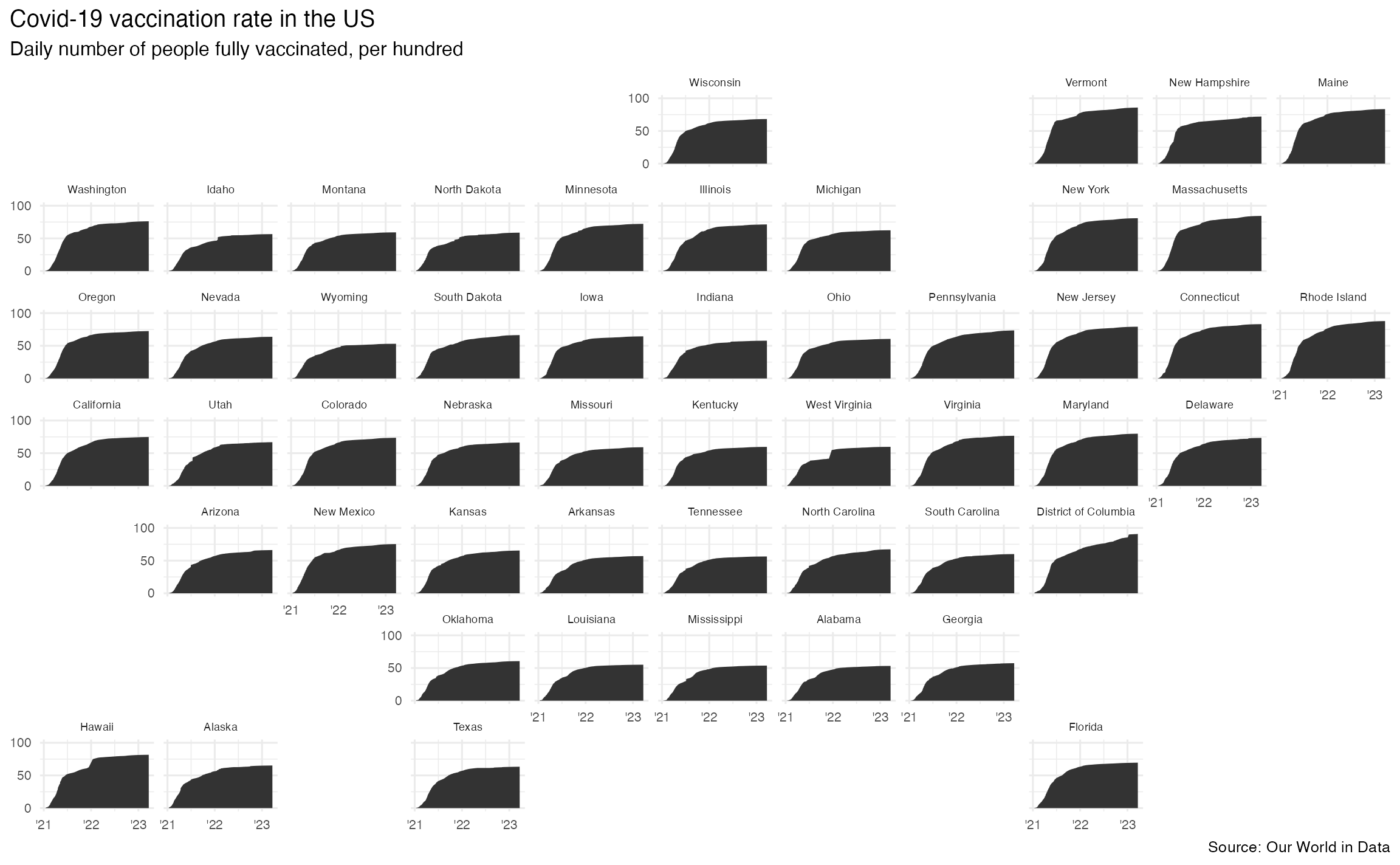
ggplot(us_state_vaccinations, aes(x = date, y = people_fully_vaccinated_per_hundred, group = location)) +
  geom_area() +
  facet_geo(facets = vars(location)) +
  scale_y_continuous(
    limits = c(0, 100),
    breaks = c(0, 50, 100),
    minor_breaks = c(25, 75)
  ) +
  scale_x_date(breaks = c(ymd("2021-01-01", "2022-01-01", "2023-01-01")), labels = c("'21", "'22", "'23")) +
  labs(
    x = NULL, y = NULL,
    title = "Covid-19 vaccination rate in the US",
    subtitle = "Daily number of people fully vaccinated, per hundred",
    caption = "Source: Our World in Data"
  ) +
  theme(
    strip.text.x = element_text(size = 7),
    axis.text = element_text(size = 8),
    plot.title.position = "plot"
  )

Daily US vaccine data by state

us_state_vaccinations <- read_csv("data/us_state_vaccinations.csv")
glimpse(us_state_vaccinations)

Rows: 51,492
Columns: 16
$ date                                <date> 2021-01-12, 2021-01-13, 2021-01-1…
$ location                            <chr> "Alabama", "Alabama", "Alabama", "…
$ total_vaccinations                  <dbl> 78134, 84040, 92300, 100567, NA, N…
$ total_distributed                   <dbl> 377025, 378975, 435350, 444650, NA…
$ people_vaccinated                   <dbl> 70861, 74792, 80480, 86956, NA, NA…
$ people_fully_vaccinated_per_hundred <dbl> 0.15, 0.19, NA, 0.28, NA, NA, NA, …
$ total_vaccinations_per_hundred      <dbl> 1.59, 1.71, 1.88, 2.05, NA, NA, NA…
$ people_fully_vaccinated             <dbl> 7270, 9245, NA, 13488, NA, NA, NA,…
$ people_vaccinated_per_hundred       <dbl> 1.45, 1.53, 1.64, 1.77, NA, NA, NA…
$ distributed_per_hundred             <dbl> 7.69, 7.73, 8.88, 9.07, NA, NA, NA…
$ daily_vaccinations_raw              <dbl> NA, 5906, 8260, 8267, NA, NA, NA, …
$ daily_vaccinations                  <dbl> NA, 5906, 7083, 7478, 7498, 7509, …
$ daily_vaccinations_per_million      <dbl> NA, 1205, 1445, 1525, 1529, 1531, …
$ share_doses_used                    <dbl> 0.207, 0.222, 0.212, 0.226, NA, NA…
$ total_boosters                      <dbl> NA, NA, NA, NA, NA, NA, NA, NA, NA…
$ total_boosters_per_hundred          <dbl> NA, NA, NA, NA, NA, NA, NA, NA, NA…

Source: https://ourworldindata.org/us-states-vaccinations

Facet by location

ggplot(
  data = us_state_vaccinations,
  mapping = aes(x = date, y = people_fully_vaccinated_per_hundred)
) +
  geom_area() +
  facet_wrap(facets = vars(location))

Data cleaning

us_state_vaccinations <- us_state_vaccinations |>
  mutate(location = if_else(location == "New York State", "New York", location)) |>
  filter(location %in% c(state.name, "District of Columbia"))

Geofacet by state

Using geofacet::facet_geo():

• Plot
• Code

ggplot(
  data = us_state_vaccinations,
  mapping = aes(x = date, y = people_fully_vaccinated_per_hundred)
) +
  geom_area() +
  facet_geo(facets = vars(location)) +
  labs(
    x = NULL, y = NULL,
    title = "Covid-19 vaccination rate in the US",
    subtitle = "Daily number of people fully vaccinated, per hundred",
    caption = "Source: Our World in Data"
  )

Geofacet by state, with improvements

• Plot
• Code

ggplot(us_state_vaccinations, aes(x = date, y = people_fully_vaccinated_per_hundred, group = location)) +
  geom_area() +
  facet_geo(facets = vars(location)) +
  scale_y_continuous(
    limits = c(0, 100),
    breaks = c(0, 50, 100),
    minor_breaks = c(25, 75)
  ) +
  scale_x_date(breaks = c(ymd("2021-01-01", "2022-01-01", "2023-01-01")), labels = c("'21", "'22", "'23")) +
  labs(
    x = NULL, y = NULL,
    title = "Covid-19 vaccination rate in the US",
    subtitle = "Daily number of people fully vaccinated, per hundred",
    caption = "Source: Our World in Data"
  ) +
  theme(
    strip.text.x = element_text(size = 7),
    axis.text = element_text(size = 8),
    plot.title.position = "plot"
  )

Bring in 2020 Presidential election results

election_2020 <- read_csv("data/us-election-2020.csv")
election_2020

# A tibble: 51 × 5
   state                electoal_votes biden trump win       
   <chr>                         <dbl> <dbl> <dbl> <chr>     
 1 Alabama                           9     0     9 Republican
 2 Alaska                            3     0     3 Republican
 3 Arizona                          11    11     0 Democrat  
 4 Arkansas                          6     0     6 Republican
 5 California                       55    55     0 Democrat  
 6 Colorado                          9     9     0 Democrat  
 7 Connecticut                       7     7     0 Democrat  
 8 Delaware                          3     3     0 Democrat  
 9 District of Columbia              3     3     0 Democrat  
10 Florida                          29     0    29 Republican
# ℹ 41 more rows

Geofacet by state, color by presidential election result

• Code
• Plot

us_state_vaccinations |>
  left_join(election_2020, by = c("location" = "state")) |>
  ggplot(mapping = aes(x = date, y = people_fully_vaccinated_per_hundred)) +
  geom_area(mapping = aes(fill = win)) +
  facet_geo(facets = vars(location)) +
  scale_y_continuous(limits = c(0, 100), breaks = c(0, 50, 100), minor_breaks = c(25, 75)) +
  scale_x_date(breaks = c(ymd("2021-01-01", "2022-01-01", "2023-01-01")), labels = c("'21", "'22", "'23")) +
  scale_fill_manual(values = c("#2D69A1", "#BD3028")) +
  labs(
    x = NULL, y = NULL,
    title = "Covid-19 vaccination rate in the US",
    subtitle = "Daily number of people fully vaccinated, per hundred",
    caption = "Source: Our World in Data",
    fill = "2020 Presidential\nElection"
  ) +
  theme(
    strip.text.x = element_text(size = 7),
    axis.text = element_text(size = 8),
    plot.title.position = "plot",
    legend.position = c(0.93, 0.15),
    legend.text = element_text(size = 9),
    legend.title = element_text(size = 11),
    legend.background = element_rect(color = "gray", size = 0.5)
  )

Wrap-up

Wrap-up

• Modern geospatial visualizations are defined by their scale, project, and symbols
• ggmap allows you to create geospatial visualizations without needing to collect the spatial features directly
• geofacet allows you to create cartograms which incorporate geographic location

The end of an era