Optimizing color spaces

Lecture 11

Dr. Benjamin Soltoff

Cornell University
INFO 3312/5312 - Spring 2024

March 2, 2023

Announcements

Announcements

• Project 1 due tomorrow by 10am
  • In-class presentations
  • Write-up
• Use the “Build” tab to render the entire website
• Carefully review project instructions

Setup

Packages + figures

# load packages
library(tidyverse)
library(readxl)
library(here)
library(patchwork)
library(knitr)
library(palmerpenguins)
library(colorblindr)
library(tidycensus)
library(scales)
library(RColorBrewer)
library(ggrepel)
library(cowplot)

# set default theme for ggplot2
theme_set(theme_minimal(base_size = 12))

YAML options

knitr:
  opts_chunk:
    fig.width: 7
    fig.asp: 0.618
    fig.retina: 2
    dpi: 150
    out.width: "80%"
    fig.showtext: true

Uses of color in data visualization

Distinguish categories (qualitative)

Qualitative scale example

• Okabe-Ito
• ColorBrewer Set1
• ColorBrewer Set3

Figure redrawn from Claus O. Wilke. Fundamentals of Data Visualization. O’Reilly, 2019.

Uses of color in data visualization

Distinguish categories (qualitative)
Represent numeric values (sequential)

Sequential scale example

• Viridis
• Inferno
• Cividis

Figure redrawn from Claus O. Wilke. Fundamentals of Data Visualization. O’Reilly, 2019.

Uses of color in data visualization

Distinguish categories (qualitative)
Represent numeric values (sequential)
Represent numeric values (diverging)

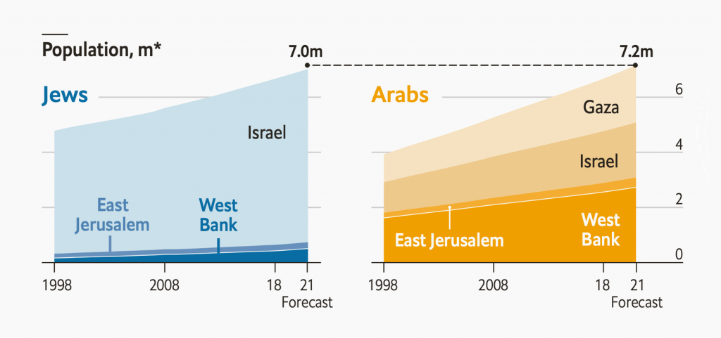
Diverging scale example

• ColorBrewer PiYG
• Carto Earth
• Blue-Red

Figure redrawn from Claus O. Wilke. Fundamentals of Data Visualization. O’Reilly, 2019.

Uses of color in data visualization

Distinguish categories (qualitative)
Represent numeric values (sequential)
Represent numeric values (diverging)
Highlight

Highlight example

• Grays with accents
• Okabe-Ito accent
• ColorBrewer accent

Figure redrawn from Claus O. Wilke. Fundamentals of Data Visualization. O’Reilly, 2019.

Uses of color in data visualization

Distinguish categories (qualitative)
Represent numeric values (sequential)
Represent numeric values (diverging)
Highlight

Choosing a color scale

Choosing a color scale

• Emphasis on interpretability and accessibility
• Default palettes are less than desirable
• Variables may require transformations

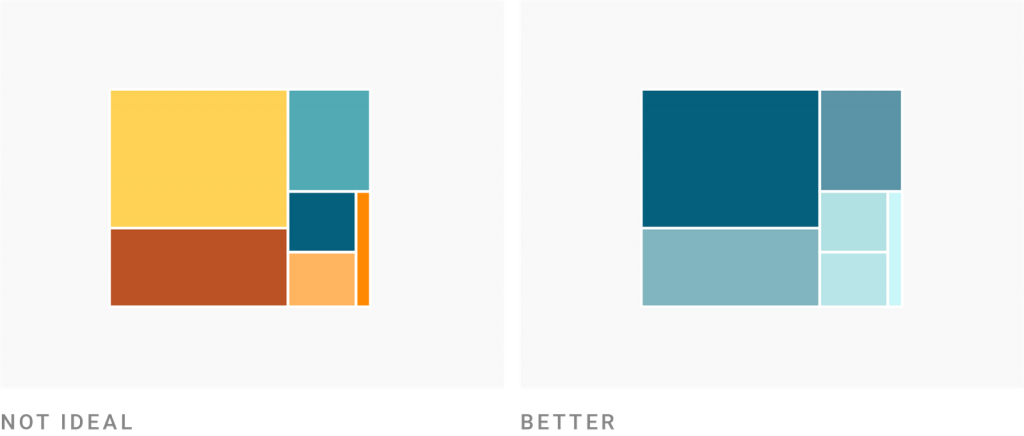
Default palette in ggplot2

Suboptimal default choices

Common forms of color vision deficiency

Red-green

• Deuteranomaly
• Protanomaly
• Protanopia and deuteranopia

Blue-yellow

• Tritanomaly
• Tritanopia

Complete color vision deficiency

• Monochromacy

Inspecting for color vision deficiency

Inspecting for color vision deficiency

library(colorblindr)
cvd_grid(plot = pen_fig)

Inspecting for color deficiency

Inspecting for color deficiency

When to use quantitative or qualitative color scales?

• Quantitative \(\equiv\) numerical
• Qualitative \(\equiv\) categorical

Source: Lisa Charlotte Muth

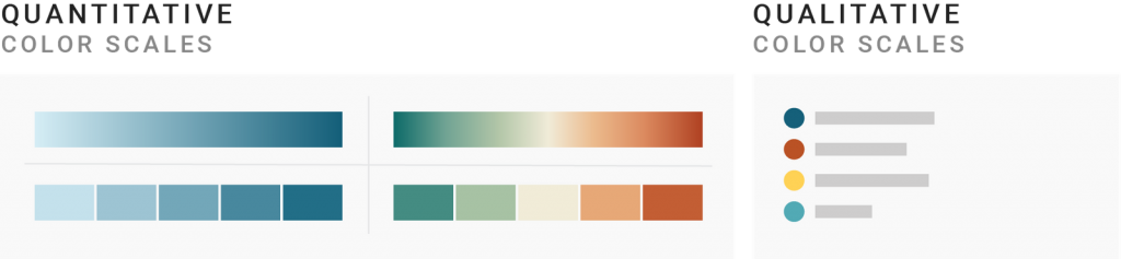
Use qualitative for nominal variables

Source: Lisa Charlotte Muth

Use quantitative for ordinal variables

Source: Lisa Charlotte Muth

Quantitative \(\neq\) continuous

Source: Lisa Charlotte Muth

Shades to emphasize order

Source: Lisa Charlotte Muth

Shades to distinguish subcategories

Source: Lisa Charlotte Muth

Implementing optimal color palettes in R

ggplot2 color scale functions

Scale function	Aesthetic	Data type	Palette type
scale_color_hue()	color	discrete	qualitative

ggplot2 color scale functions are a bit of a mess

Scale function	Aesthetic	Data type	Palette type
scale_color_hue()	color	discrete	qualitative
scale_fill_hue()	fill	discrete	qualitative

ggplot2 color scale functions are a bit of a mess

Scale function	Aesthetic	Data type	Palette type
scale_color_hue()	color	discrete	qualitative
scale_fill_hue()	fill	discrete	qualitative
scale_color_gradient()	color	continuous	sequential

ggplot2 color scale functions are a bit of a mess

Scale function	Aesthetic	Data type	Palette type
scale_color_hue()	color	discrete	qualitative
scale_fill_hue()	fill	discrete	qualitative
scale_color_gradient()	color	continuous	sequential
scale_color_gradient2()	color	continuous	diverging

ggplot2 color scale functions are a bit of a mess

Scale function	Aesthetic	Data type	Palette type
scale_color_hue()	color	discrete	qualitative
scale_fill_hue()	fill	discrete	qualitative
scale_color_gradient()	color	continuous	sequential
scale_color_gradient2()	color	continuous	diverging
scale_fill_viridis_c()	color	continuous	sequential
scale_fill_viridis_d()	fill	discrete	sequential
scale_color_brewer()	color	discrete	qualitative, diverging, sequential
scale_fill_brewer()	fill	discrete	qualitative, diverging, sequential
scale_color_distiller()	color	continuous	qualitative, diverging, sequential

… and there are many many more

Examples

ggplot(temps_months, aes(x = month, y = location, fill = mean)) + 
  geom_tile(width = 0.95, height = 0.95) + 
  coord_fixed(expand = FALSE) +
  theme_classic()

Examples

ggplot(temps_months, aes(x = month, y = location, fill = mean)) + 
  geom_tile(width = 0.95, height = 0.95) + 
  coord_fixed(expand = FALSE) +
  theme_classic() +
  scale_fill_gradient()

Examples

ggplot(temps_months, aes(x = month, y = location, fill = mean)) + 
  geom_tile(width = 0.95, height = 0.95) + 
  coord_fixed(expand = FALSE) +
  theme_classic() +
  scale_fill_viridis_c()

Examples

ggplot(temps_months, aes(x = month, y = location, fill = mean)) + 
  geom_tile(width = 0.95, height = 0.95) + 
  coord_fixed(expand = FALSE) +
  theme_classic() +
  scale_fill_viridis_c(option = "B", begin = 0.15)

Examples

ggplot(temps_months, aes(x = month, y = location, fill = mean)) + 
  geom_tile(width = 0.95, height = 0.95) + 
  coord_fixed(expand = FALSE) +
  theme_classic() +
  scale_fill_distiller(palette = "YlGnBu")

The colorspace package creates some order

Scale name: scale_<aesthetic>_<datatype>_<colorscale>()

• <aesthetic>: name of the aesthetic (fill, color, colour)
• <datatype>: type of variable plotted (discrete, continuous, binned)
• <colorscale>: type of the color scale (qualitative, sequential, diverging, divergingx)

Scale function	Aesthetic	Data type	Palette type
scale_color_discrete_qualitative()	color	discrete	qualitative
scale_fill_continuous_sequential()	fill	continuous	sequential
scale_colour_continuous_divergingx()	colour	continuous	diverging

Examples

ggplot(temps_months, aes(x = month, y = location, fill = mean)) + 
  geom_tile(width = 0.95, height = 0.95) + 
  coord_fixed(expand = FALSE) +
  theme_classic() +
  scale_fill_continuous_sequential(palette = "YlGnBu")

Examples

ggplot(temps_months, aes(x = month, y = location, fill = mean)) + 
  geom_tile(width = 0.95, height = 0.95) + 
  coord_fixed(expand = FALSE) +
  theme_classic() +
  scale_fill_continuous_sequential(palette = "Viridis")

Examples

ggplot(temps_months, aes(x = month, y = location, fill = mean)) + 
  geom_tile(width = 0.95, height = 0.95) + 
  coord_fixed(expand = FALSE) +
  theme_classic() +
  scale_fill_continuous_sequential(palette = "Inferno", begin = 0.15)

Setting colors for discrete, qualitative scales

Examples

ggplot(popgrowth, aes(x = pop2000, y = popgrowth, color = region)) +
  geom_point(size = 4) +
  scale_x_log10()

Examples

ggplot(popgrowth, aes(x = pop2000, y = popgrowth, color = region)) +
  geom_point(size = 4) +
  scale_x_log10() +
  scale_color_hue()

Examples

ggplot(popgrowth, aes(x = pop2000, y = popgrowth, color = region)) +
  geom_point(size = 4) +
  scale_x_log10() +
  scale_color_discrete_qualitative(palette = "Dark 2")

Examples

library(ggthemes)  # for scale_color_colorblind()

ggplot(popgrowth, aes(x = pop2000, y = popgrowth, color = region)) +
  geom_point(size = 4) +
  scale_x_log10() +
  scale_color_colorblind()

Examples

ggplot(popgrowth, aes(x = pop2000, y = popgrowth, color = region)) +
  geom_point(size = 4) +
  scale_x_log10() +
  scale_color_manual(
    values = c(
      West = "#E69F00", South = "#56B4E9",
      Midwest = "#009E73", Northeast = "#F0E442"
    )
  )

Okabe-Ito RGB codes

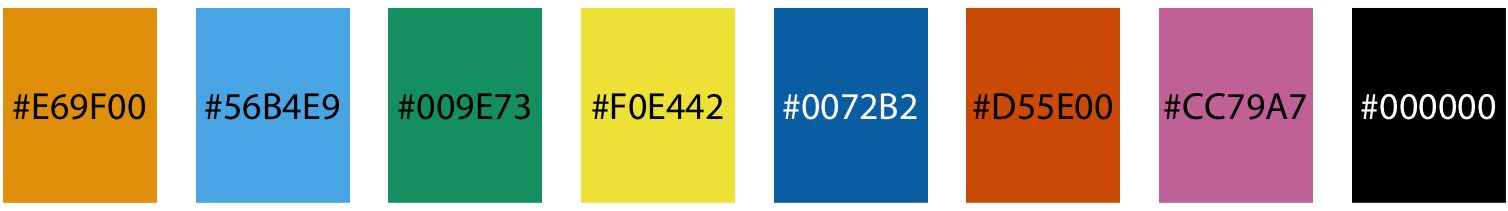
Name	Hex code	R, G, B (0-255)
orange	#E69F00	230, 159, 0
sky blue	#56B4E9	86, 180, 233
bluish green	#009E73	0, 158, 115
yellow	#F0E442	240, 228, 66
blue	#0072B2	0, 114, 178
vermilion	#D55E00	213, 94, 0
reddish purple	#CC79A7	204, 121, 167
black	#000000	0, 0, 0

ae-colorspace

• Go to the course GitHub org and find your ae-colorspace (repo name will be suffixed with your GitHub name).
• Clone the repo in RStudio Workbench, open the Quarto document in the repo, and follow along and complete the exercises.